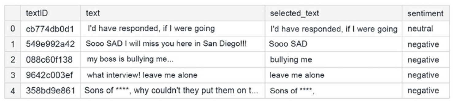
1. Introduction• Natural language processing (NLP) is a field operating at the intersection of linguistics, computer science, and AI.• Its primary focus is algorithms to process and analyze large amounts of natural language data.2. Sentiment Analysis• Sentiment analysis as a simple classification problem is extremely popular and discussed all over NLP literature.• Here, we begin with a somewhat more interesting variation on the problem: identifying sentiment-supporting phrases in a tweet.– In other words, it is important not to just decide on the sentiment, but also to be able to investigate the how: which words actually led to the sentiment description?2.1. Data Preparation• We will demonstrate an approach to this problem by using data from the Tweet Sentiment Extraction competition.
• Note: The selected_text column denotes the support phrase which is the part of the tweet that was the basis for the decision on sentiment assignment.
Figure 1:Sample rows from the training data
• Now, we perform some basic clean ups:
# get rid of website URLs and non-characters and replace the stars people use in place of swear words with a single token, "swear".defbasic_cleaning(text): text=re.sub(r'https?://www\.\S+\.com','',text) text=re.sub(r'[^A-Za-z|\s]','',text) text=re.sub(r'\*+','swear',text)# Capture swear words that are **** outreturn text# remove HTML from the content of the tweetsdefremove_html(text): html=re.compile(r'<.*?>')return html.sub(r'',text)defremove_emoji(text): emoji_pattern = re.compile("["u"\U0001F600-\U0001F64F"#emoticonsu"\U0001F300-\U0001F5FF"#symbols & pictographsu"\U0001F680-\U0001F6FF"#transport & map symbolsu"\U0001F1E0-\U0001F1FF"#flags (iOS)u"\U00002702-\U000027B0"u"\U000024C2-\U0001F251""]+", flags=re.UNICODE)return emoji_pattern.sub(r'', text)# remove repeating characters; e.g. so taht we have "way" instead of "waaayyyy"defremove_multiplechars(text): text = re.sub(r'(.)\1{3,}',r'\1', text)return text
• For convenience, we can combine all of these clean up functions into one:
• The last bit of preparation involves writing functions for creating the embeddings based on a pre-trained model (the tokenizer argument):
deffast_encode(texts, tokenizer, chunk_size=256, maxlen=128): tokenizer.enable_truncation(max_length=maxlen) tokenizer.enable_padding(max_length=maxlen) all_ids =[]for i inrange(0,len(texts), chunk_size): text_chunk = texts[i:i+chunk_size].tolist() encs = tokenizer.encode_batch(text_chunk) all_ids.extend([enc.ids for enc in encs])return np.array(all_ids)
• Next, we create a pre-processing function enabling us to work with the entire corpus:
defpreprocess_news(df,stop=stop,n=1,col='text'):'''Function to preprocess and create corpus''' new_corpus=[] stem=PorterStemmer() lem=WordNetLemmatizer()for text in df[col]: words=[w for w in word_tokenize(text)if(w notin stop)] words=[lem.lemmatize(w)for w in words if(len(w)>n)] new_corpus.append(words) new_corpus=[word for l in new_corpus for word in l]return new_corpus
• The sentiment column is our target, and we convert it to dummy variables (one-hot encoding) for performance:
• A necessary next step is tokenization of the input texts, as well as conversion into sequences (along with padding, to ensure equal lengths across the dataset):
• We will create the embeddings for our model using DistilBERT and use them as-is.– DistilBERT is a lightweight version of BERT: the tradeoff is 3% performance loss at 40% fewer parameters.– Note: We could train the embedding layer and gain performance – at the cost of massively increased training time.
import transformersfrom tokenizers import BertWordPieceTokenizertokenizer = transformers.AutoTokenizer.from_pretrained("distilbert-base-uncased")# Save the loaded tokenizer locallysave_path ='/kaggle/working/distilbert_base_uncased/'ifnot os.path.exists(save_path): os.makedirs(save_path)tokenizer.save_pretrained(save_path)# Reload it with the huggingface tokenizers libraryfast_tokenizer = BertWordPieceTokenizer('distilbert_base_uncased/vocab.txt', lowercase=True)fast_tokenizer
• We can use the previously defined fast_encode function, along with the fast_tokenizer defined above, to encode the tweets:
X = fast_encode(df_clean_selection.text.astype(str), fast_tokenizer, maxlen=128)
• With the data prepared, we can construct the model.2.2. Model• We go with a fairly standard architecture: a combination of LSTM layers, normalized by global pooling and dropout, and a dense layer on top.
2.3. Prediction• Generating a prediction from the fitted model proceeds in a straightforward manner. In order to utilize all the available data, we begin by re-training our model on all available data (so no validation):
df_clean_final = df_clean.sample(frac=1)X_train = fast_encode(df_clean_selection.text.astype(str), fast_tokenizer, maxlen=128)y_train = y
• We refit the model on the entire dataset before generating the predictions:
y_preds = model_DistilBert.predict(X_test)y_predictions = pd.DataFrame(y_preds, columns=['negative','neutral','positive'])y_predictions_final = y_predictions.idxmax(axis=1)accuracy = accuracy_score(y_test,y_predictions_final)print(f"The final model shows {accuracy:.2f} accuracy on the test set.")
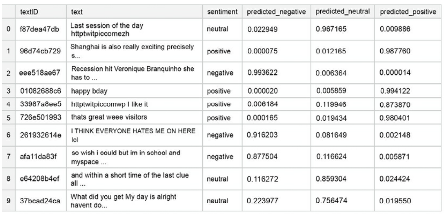
• The final model shows 0.74 accuracy on the test set. Below we show a sample of what the output looks like:
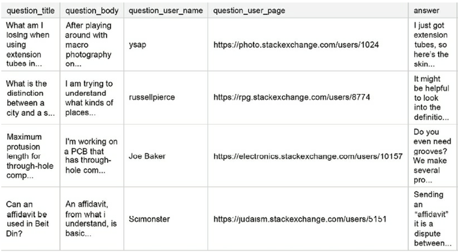
• You can see already from these few rows, there are some instances where the sentiment is obvious to a human reader, but the model fails to capture it.2.4. Improvements• There are some improvements that can be made if you want to achieve competitive performance, given below in order of likely impact:– Larger embeddings: This allows us to capture more information already at the (processed) input data level.– Bigger model: More units in the LSTM layers.– Longer training: i.e. more epochs2.5. Pipeline• While the improvements listed above will undoubtedly boost the performance of the model, the core elements of our pipeline are reusable:– Data cleaning and pre-processing– Creating text embeddings– Incorporating recurrent layers and regularization in the target model architecture.3. Open Domain Q&A• In this section, we'll be looking at the Google QUEST Q&A Labeling competition.– In this competition, question-answer pairs were evaluated by human raters on a diverse set of criteria, such as “question conversational,” “question fact-seeking,” or “answer helpful.”– The task was to predict a numeric value for each of the target columns (i.e. corresponding to the criteria).– Note: Since the labels were aggregated across multiple raters, the objective was effectively a multivariate regression output, with target columns normalized to the unit range.– Note: The metric used in the competition was Spearman correlation (linear correlation computed on ranks).3.1. Baseline Model• Before engaging in modeling with advanced techniques (like transformer-based models for NLP), it is frequently a good idea to establish a baseline with simpler methods.3.1.1. Helper Functions• We begin by defining several helper functions, which can help us extract different aspects of the text. • First, a function that will output a word count given a string:
• Since we intend to build a Scikit-learn pipeline, it is useful to define the metric as a scorer.– The make_scorer method is a wrapper in Scikit-learn that takes a scoring function, like accuracy or MSE, and returns a callable that scores an output of the estimator.–
• Next, a small helper function to extract successive chunks of size n from l.– This will help us later with generating embeddings for our body of text without running into memory problems:
defchunks(l, n):for i inrange(0,len(l), n):yield l[i:i + n]
3.1.2. Preparing Data• Part of the feature set we will use is embeddings from pre-trained models.– Although we are building a baseline, we still can use pre-trained models.• We begin by importing the tokenizer and model, and then we process the corpus in chunks, encoding each question/answer into a fixed-size embedding:
deffetch_vectors(string_list, batch_size=64):# Inspired by https://jalammar.github.io/a-visual-guide-to-using-bert- for-the-first-time/ DEVICE = torch.device("cuda") tokenizer = transformers.DistilBertTokenizer.from_pretrained("../input/distilbertbaseuncased/") model = transformers.DistilBertModel.from_pretrained("../input/distilbertbaseuncased/") model.to(DEVICE) fin_features =[]for data in chunks(string_list, batch_size): tokenized =[]for x in data: x =" ".join(x.strip().split()[:300]) tok = tokenizer.encode(x, add_special_tokens=True) tokenized.append(tok[:512]) max_len =512 padded = np.array([i +[0]*(max_len -len(i))for i in tokenized]) attention_mask = np.where(padded !=0,1,0) input_ids = torch.tensor(padded).to(DEVICE) attention_mask = torch.tensor(attention_mask).to(DEVICE)with torch.no_grad(): last_hidden_states = model(input_ids, attention_mask=attention_mask) features = last_hidden_states[0][:,0,:].cpu().numpy() fin_features.append(features) fin_features = np.vstack(fin_features)return fin_features
3.1.3. Feature Engineering• We start by counting the words in the title and body of the question, as well as the answer. This is a simple yet surprisingly useful feature in many applications:
• When dealing with information sourced from online, we can extract potentially informative features by examining the components of a website address (where we define components as elements of the address separated by dots).– We count the number of components, and store individual ones as features:
for df in[xtrain, xtest]: df['domcom']= df['question_user_page'].apply(lambda s: s.split('://')[1].split('/')[0].split('.'))# Count components df['dom_cnt']= df['domcom'].apply(lambda s:len(s))# Pad the length in case some domains have fewer components in the name df['domcom']= df['domcom'].apply(lambda s: s +['none','none'])# Componentsfor ii inrange(0,4): df['dom_'+str(ii)]= df['domcom'].apply(lambda s: s[ii])
• Numerous target columns deal with how relevant the answer is for a given question. One possible way of quantifying this relationship is evaluating shared words within a pair of strings:
# Shared elementsfor df in[xtrain, xtest]: df['q_words']= df['question_body'].apply(lambda s:[f for f in s.split()if f notin eng_stopwords]) df['a_words']= df['answer'].apply(lambda s:[f for f in s.split()if f notin eng_stopwords]) df['qa_word_overlap']= df.apply(lambda s:len(np.intersect1d(s['q_words'], s['a_words'])), axis =1) df['qa_word_overlap_norm1']= df.apply(lambda s: s['qa_word_overlap']/(1+len(s['a_words'])), axis =1) df['qa_word_overlap_norm2']= df.apply(lambda s: s['qa_word_overlap']/(1+len(s['q_words'])), axis =1) df.drop(['q_words','a_words'], axis =1, inplace =True)
• Stopwords and punctuation occurrence patterns can tell us something about the style and intent:
for df in[xtrain, xtest]:## Number of characters in the text ## df["question_title_num_chars"]= df["question_title"].apply(lambda x:len(str(x))) df["question_body_num_chars"]= df["question_body"].apply(lambda x:len(str(x))) df["answer_num_chars"]= df["answer"].apply(lambda x:len(str(x)))## Number of stopwords in the text ## df["question_title_num_stopwords"]= df["question_title"].apply(lambda x:len([w for w instr(x).lower().split()if w in eng_stopwords])) df["question_body_num_stopwords"]= df["question_body"].apply(lambda x:len([w for w instr(x).lower().split()if w in eng_stopwords])) df["answer_num_stopwords"]= df["answer"].apply(lambda x:len([w for w instr(x).lower().split()if w in eng_stopwords]))## Number of punctuations in the text ## df["question_title_num_punctuations"]=df['question_title'].apply(lambda x:len([c for c instr(x)if c in string.punctuation])) df["question_body_num_punctuations"]=df['question_body'].apply(lambda x:len([c for c instr(x)if c in string.punctuation])) df["answer_num_punctuations"]=df['answer'].apply(lambda x:len([c for c instr(x)if c in string.punctuation]))## Number of title case words in the text ## df["question_title_num_words_upper"]= df["question_title"].apply(lambda x:len([w for w instr(x).split()if w.isupper()])) df["question_body_num_words_upper"]= df["question_body"].apply(lambda x:len([w for w instr(x).split()if w.isupper()])) df["answer_num_words_upper"]= df["answer"].apply(lambda x:len([w for w instr(x).split()if w.isupper()]))
3.1.4. Creating Embeddings• With the “vintage” features prepared – where our focus is on simple summary statistics of the text, without paying heed to semantic structure – we can move on to creating embeddings for the questions and answers.• We could theoretically train a separate word2vec-type model on our data (or fine-tune an existing one), but for the sake of this presentation we will use a pre-trained model as is.• A useful choice is the Universal Sentence Encoder from Google.– This model is trained on a variety of data sources. It takes as input a piece of text in English and outputs a 512-dimensional vector.
• The code for turning the text fields into embeddings is presented below: – We loop through the entries in the training/test sets in batches, embed each batch (for memory efficiency reasons).– Then append them to the original list. – The final data frames are constructed by stacking each list of batch-level embeddings vertically.
embeddings_train ={}embeddings_test ={}for text in['question_title','question_body','answer']: train_text = xtrain[text].str.replace('?','.').str.replace('!','.').tolist() test_text = xtest[text].str.replace('?','.').str.replace('!','.').tolist() curr_train_emb =[] curr_test_emb =[] batch_size =4 ind =0while ind*batch_size <len(train_text): curr_train_emb.append(embed(train_text[ind*batch_size:(ind +1)*batch_size])["outputs"].numpy()) ind +=1 ind =0while ind*batch_size <len(test_text): curr_test_emb.append(embed(test_text[ind*batch_size:(ind +1)*batch_size])["outputs"].numpy()) ind +=1 embeddings_train[text +'_embedding']= np.vstack(curr_train_emb) embeddings_test[text +'_embedding']= np.vstack(curr_test_emb)print(text)
• Given the vector representations for both questions and answers, we can calculate the semantic similarity between the fields by using different distance metrics on the pairs of vectors. • Theidea behind trying different metrics is the desire to capture diverse types of characteristics; an analogy in the context of classification would be to use both accuracy and entropy to get a complete picture of the situation:
• Let's gather the distance features in separate columns:
for ii inrange(0,6): xtrain['dist'+str(ii)]= dist_features_train[:,ii] xtest['dist'+str(ii)]= dist_features_test[:,ii]
• Finally, we can also create TF-IDF representations of the text fields. – The general idea is to create multiple features based on diverse transformations of the input text, and then feed them to a relatively simple model. – This way, we can capture the characteristics of the data without the need to fit a sophisticated deep learning model. – We can achieve it by analyzing the text at the word as well as the character level. – To limit the memory consumption, we put an upper bound on the maximum number of both kinds of features (your mileage might vary; with more memory, these limits can be upped):
limit_char =5000limit_word =25000
• We instantiate character- and word-level vectorizers. – Note: The setup of our problem lends itself to a convenient usage of the Pipeline functionality from Scikit-learn, allowing a combination of multiple steps in the model fitting procedure. • We begin by creating two separate transformers for the title column (word- and character-level):
3.1.5. Numerical Features• We wrap up the feature engineering part by processing the numerical features. • We use simple methods only: – Missing value imputation to take care of N/A values and – A power transformer to stabilize the distribution and make it closer to Gaussian (which is frequently helpful if you are using a numerical feature inside a neural network):
3.1.6. Handling Categorical Variables• A useful feature of Pipelines is they can be combined and nested. • Next, we add functionality to handle categorical variables, and then put it all together in a ColumnTransformer object to streamline the data pre-processing and feature engineering logic. • Each part of the input can be handled in its own appropriate manner:
3.1.8. Model Validation• It is always a good idea to evaluate the performance of your model out of sample: a convenient way to go about this is to create out-of-fold predictions.• The procedure involves the following steps:(a) Split the data into folds. In our case we use GroupKFold, since one question can have multiple answers (in separate rows of the data frame). In order to prevent information leakage, we want to ensure each question only appears in one fold.(b) For each fold, train the model using the data in the other folds, and generate the predictions for the fold of choice, as well as the test set.(c) Average the predictions on the test set.• We start with preparing the “storage” matrices in which we will store the predictions.– mvalid will contain the out-of-fold predictions, while mfull is a placeholder for the predictions on the entire test set, averaged across folds. – Since several questions contain more than one candidate answer, we stratify our KFold split on question_body:
nfolds =5mvalid = np.zeros((xtrain.shape[0],len(target_cols)))mfull = np.zeros((xtest.shape[0],len(target_cols)))kf = GroupKFold(n_splits= nfolds).split(X=xtrain.question_body, groups=xtrain.question_body)# Loop through the folds and build the separate modelsfor ind,(train_index, test_index)inenumerate(kf):# Split the data into training and validation x0, x1 = xtrain.loc[train_index], xtrain.loc[test_index] y0, y1 = ytrain.loc[train_index], ytrain.loc[test_index]for ii inrange(0, ytrain.shape[1]):# Fit model be = clone(pipeline) be.fit(x0, np.array(y0)[:,ii]) filename ='ridge_f'+str(ind)+'_c'+str(ii)+'.pkl' pickle.dump(be,open(filename,'wb'))# Storage matrices for the OOF and test predictions, respectively mvalid[test_index, ii]= be.predict(x1) mfull[:,ii]+= be.predict(xtest)/nfoldsprint('---')
• Once the fitting part is done, we can evaluate the performance in accordance with the metric specified in the competition:
• The final score is 0.34, which is fairly acceptable as a starting point.Note:In this section, we have demonstrated how to build descriptive features on a body of text. While this is not a winning formula for an NLP competition (the score is OK, but not a guarantee for landing in the medal zone), it is a useful tool to keep in your toolbox. 4. Text Augmentation Strategies4.1. Basic Techniques• A systematic study of the basic approaches is provided in Wei and Zou (2019).4.1.1. Synonym Replacement• Replacing certain words with their synonyms produces text that is close in meaning to the original, but slightly perturbed (see the project page for more details, like where the synonyms are actually coming from).
defget_synonyms(word): synonyms =set()for syn in wordnet.synsets(word):for l in syn.lemmas(): synonym = l.name().replace("_"," ").replace("-"," ").lower() synonym ="".join([char for char in synonym if char in' qwertyuiopasdfghjklzxcvbnm']) synonyms.add(synonym)if word in synonyms: synonyms.remove(word)returnlist(synonyms)
• We create a simple wrapper around the workhorse function defined above, specifying a chunk of text (a string containing multiple words) and replace at most n of the words:
defsynonym_replacement(words, n): words = words.split() new_words = words.copy() random_word_list =list(set([word for word in words if word notin stop_words])) random.shuffle(random_word_list) num_replaced =0for random_word in random_word_list: synonyms = get_synonyms(random_word)iflen(synonyms)>=1: synonym = random.choice(list(synonyms)) new_words =[synonym if word == random_word else word for word in new_words] num_replaced +=1if num_replaced >= n:# Only replace up to n wordsbreak sentence =' '.join(new_words)return sentence
# Let's see how this function worksprint(f" Example of Synonym Replacement: {synonym_replacement('The quick brown fox jumps over the lazy dog',4)}")Example of Synonym Replacement: The spry brown university fox jumpstart over the lazy detent
• Not quite what you would call Shakespearean, but it does convey the same message while changing the style markedly.• We can extend this approach by creating multiple new sentences per tweet:
trial_sent = data['text'][25]print(trial_sent)the free fillin' app on my ipod is fun, im addictedfor n inrange(3):print(f" Example of Synonym Replacement: {synonym_replacement(trial_sent,n)}")
Example of Synonym Replacement: the free fillin' app on my ipod is fun, im addictExample of Synonym Replacement: the innocent fillin' app on my ipod is fun, im addictedExample of Synonym Replacement: the relinquish fillin' app on my ipod is fun, im addict
4.1.2. Swapping• Swapping is a simple and efficient method; we create a modified sentence by randomly swapping the order of words in the text.• Note: Carefully applied, this can be viewed as a potentially useful form of regularization, as it disturbs the sequential nature of the data that models like LSTM rely on.• The first step is to define a function swapping words:
# n is the number of words to be swappeddefrandom_swap(words, n): words = words.split() new_words = words.copy()for _ inrange(n): new_words = swap_word(new_words) sentence =' '.join(new_words)return sentence
4.1.3. Adding/Removing Words• Synonyms and swapping do not affect the length of the sentence we are modifying. • If in a given application it is useful to modify that attribute, we can remove or add words to the sentence. • The most common way to implement the former is to delete words at random:
defrandom_deletion(words, p): words = words.split()# Obviously, if there's only one word, don't delete itiflen(words)==1:return words# Randomly delete words with probability p new_words =[]for word in words: r = random.uniform(0,1)if r > p: new_words.append(word)# If you end up deleting all words, just return a random wordiflen(new_words)==0: rand_int = random.randint(0,len(words)-1)return[words[rand_int]] sentence =' '.join(new_words)return sentence
print(random_deletion(trial_sent,0.2))print(random_deletion(trial_sent,0.3))print(random_deletion(trial_sent,0.4))the free fillin' app on my is fun, addictedfree fillin' app on my ipod is im addictedthe free on my ipod is fun, im
• If we can remove, we can also add, of course. Random insertion of words to a sentence can be viewed as the NLP equivalent of adding noise or blur to an image:
print(random_insertion(trial_sent,1))print(random_insertion(trial_sent,2))print(random_insertion(trial_sent,3))the free fillin' app on my addict ipod is fun, im addictedthe complimentary free fillin' app on my ipod along is fun, im addictedthe free along fillin' app addict on my ipod along is fun, im addicted
• We can combine all the transformations discussed above into a single function, producing four variants of the same sentence:
defaug(sent,n,p):print(f" Original Sentence : {sent}")print(f" SR Augmented Sentence : {synonym_replacement(sent,n)}")print(f" RD Augmented Sentence : {random_deletion(sent,p)}")print(f" RS Augmented Sentence : {random_swap(sent,n)}")print(f" RI Augmented Sentence : {random_insertion(sent,n)}")aug(trial_sent,4,0.3)Original Sentence : the free fillin' app on my ipod is fun, im addictedSR Augmented Sentence : the disembarrass fillin' app on my ipod is fun, im hookRD Augmented Sentence : the free app on my ipod fun, im addictedRS Augmented Sentence : on free fillin' ipod is my the app fun, im addictedRI Augmented Sentence : the free fillin' app on gratis addict my ipod is complimentary make up fun, im addicted
Note:The augmentation methods discussed above do not exploit the structure of text data - to give one example, even analyzing a simple characteristic like “part of speech” can help us construct more useful transformations of the original text. This is the approach we will now focus on.4.2. nlpaug• We conclude this section by demonstrating the capabilities provided by the nlpaugpackage.– pip install nlpaug– It aggregates different methods for text augmentation and is designed to be lightweight and easy to incorporate into a workflow.• We import the character- and word-level augmenters, which we will use to plug in specific methods:
import nlpaug.augmenter.char as nacimport nlpaug.augmenter.word as nawtest_sentence ="I genuinely have no idea what the output of this sequence of words will be - it will be interesting to find out what nlpaug can do with this!"
4.2.1. Simulated Typo• What happens when we apply a simulated typo to our test sentence?– This transformation can be parametrized in a number of ways.– Note: For a full list of parameters and their explanations, examine the official documentation.
aug = nac.KeyboardAug(name='Keyboard_Aug', aug_char_min=1, aug_char_max=10, aug_char_p=0.3, aug_word_p=0.3, aug_word_min=1, aug_word_max=10, stopwords=None, tokenizer=None, reverse_tokenizer=None, include_special_char=True, include_numeric=True, include_upper_case=True, lang='en', verbose=0, stopwords_regex=None, model_path=None, min_char=4)test_sentence_aug = aug.augment(test_sentence)print(test_sentence)print(test_sentence_aug)# outputI genuinely have no idea what the output of this sequence of words will be - it will be interesting to find out what nlpaug can do with this!I geb&ine:y have no kdeZ qhQt the 8uYput of tTid sequsnDr of aorVs will be - it wi,k be jnterewtlHg to find out what nlpaug can do with this!
4.2.2. OCR Error• We can simulate an OCR error creeping into our input:
aug = nac.OcrAug(name='OCR_Aug', aug_char_min=1, aug_char_max=10, aug_char_p=0.3, aug_word_p=0.3, aug_word_min=1, aug_word_max=10, stopwords=None, tokenizer=None, reverse_tokenizer=None, verbose=0, stopwords_regex=None, min_char=1)test_sentence_aug = aug.augment(test_sentence)print(test_sentence)print(test_sentence_aug)# outputI genuinely have no idea what the output of this sequence of words will be - it will be interesting to find out what nlpaug can do with this!I 9enoine1y have no idea what the ootpot of this sequence of wokd8 will be - it will be inteke8tin9 to find out what nlpaug can du with this!
4.2.3. Word-level Modifications• While useful, character-level transformations have a limited scope when it comes to creative changes in the data. • Let us examine what possibilities nlpaug offers when it comes to word-level modifications. • Our first example is replacing a fixed percentage of words with their antonyms:
aug = naw.AntonymAug(name='Antonym_Aug', aug_min=1, aug_max=10, aug_p=0.3, lang='eng', stopwords=None, tokenizer=None, reverse_tokenizer=None, stopwords_regex=None, verbose=0)test_sentence_aug = aug.augment(test_sentence)print(test_sentence)print(test_sentence_aug)# outputI genuinely have no idea what the output of this sequence of words will be - it will be interesting to find out what nlpaug can do with this!I genuinely lack no idea what the output of this sequence of words will differ - it will differ uninteresting to lose out what nlpaug can unmake with this!
• nlpaug also offers us a possibility for, for example, replacing synonyms; such transformations can also be achieved with the more basic techniques discussed above. • For completeness’ sake, we demonstrate a small sample below, which uses a BERT architecture under the hood:
aug = naw.ContextualWordEmbsAug(model_path='bert-base-uncased', model_type='', action='substitute',# temperature=1.0, top_k=100,# top_p=None, name='ContextualWordEmbs_Aug', aug_min=1, aug_max=10, aug_p=0.3, stopwords=None, device='cpu', force_reload=False,# optimize=None, stopwords_regex=None, verbose=0, silence=True)test_sentence_aug = aug.augment(test_sentence)print(test_sentence)print(test_sentence_aug)# outputI genuinely have no idea what the output of this sequence of words will be - it will be interesting to find out what nlpaug can do with this!i genuinely have no clue what his rest of this series of words will say - its will seemed impossible to find just what we can do with this!