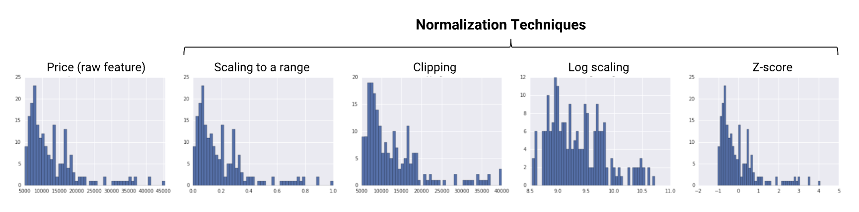
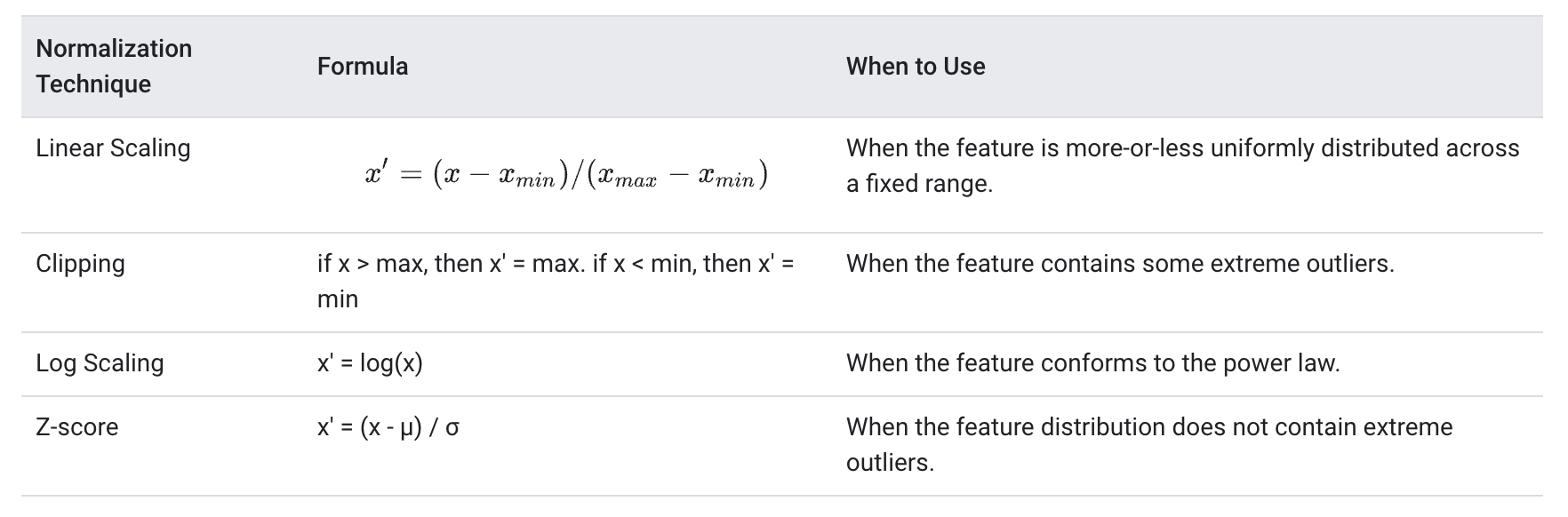
Source1. Transforming Numeric Data• You may need to apply two kinds of transformations to numeric data:– Normalizing - transforming numeric data to the same scale as other numeric data.– Bucketing - transforming numeric (usually continuous) data to categorical data.1.1. Why Normalize Numeric Features?• We strongly recommend normalizing a data set that has numeric features covering distinctly different ranges (for example, age and income). – When different features have different ranges, gradient descent can "bounce" and slow down convergence. – Optimizers like Adagrad and Adam protect against this problem by creating a separate effective learning rate for each feature.• We also recommend normalizing a single numeric feature that covers a wide range, such as "city population." – If you don't normalize the "city population" feature, training the model might generate NaN errors. – Unfortunately, optimizers like Adagrad and Adam can't prevent NaN errors when there is a wide range of values within a single feature.1.2. Normalization• The goal of normalization is to transform features to be on a similar scale. This improves the performance and training stability of the model.• Four common normalization techniques may be useful:– scaling to a range– clipping– log scaling– z-score• The following charts show the effect of each normalization technique on the distribution of the raw feature (price) on the left.
Figure 1:Summary of Normalization Techniques
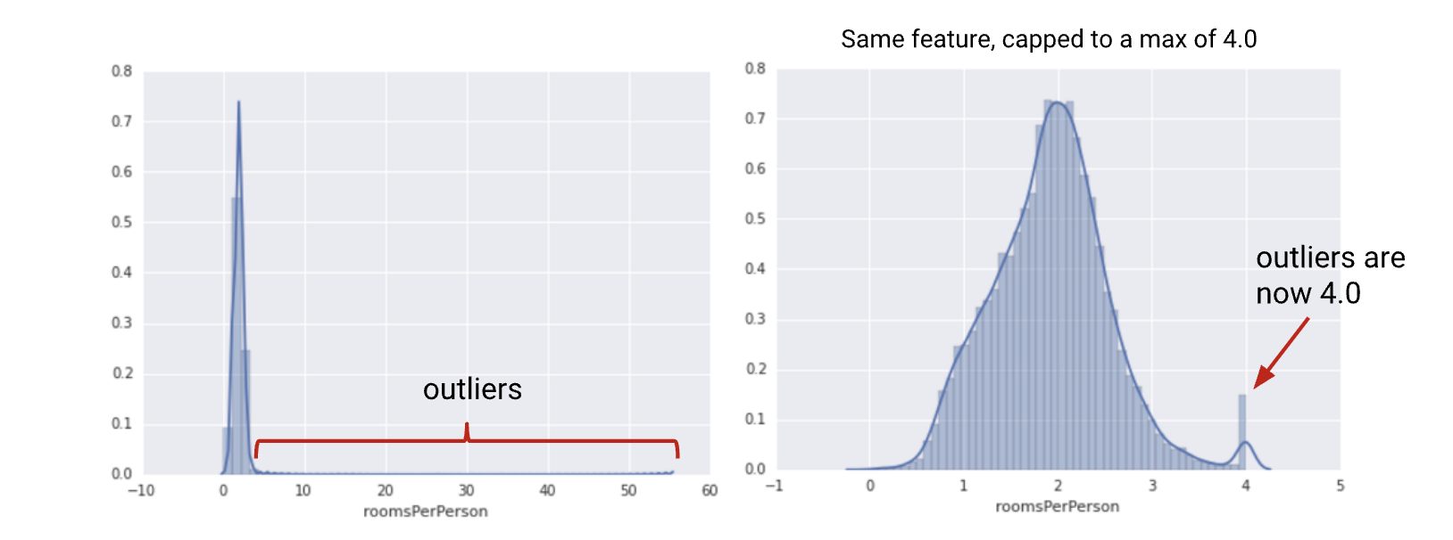
1.2.1. Scaling to a range• Scaling means converting floating-point feature values from their natural range (for example, 100 to 900) into a standard range—usually 0 and 1 (or sometimes -1 to +1). Use the following simple formula to scale to a range:x′=(x-xmin)⁄(xmax-xmin)• Scaling to a range is a good choice when both of the following conditions are met:– You know the approximate upper and lower bounds on your data with few or no outliers.– Your data is approximately uniformly distributed across that range.– A good example is age. Most age values falls between 0 and 90, and every part of the range has a substantial number of people.– In contrast, you would not use scaling on income, because only a few people have very high incomes. The upper bound of the linear scale for income would be very high, and most people would be squeezed into a small part of the scale.1.2.2. Feature Clipping• If your data set contains extreme outliers, you might try feature clipping, which caps all feature values above (or below) a certain value to fixed value. For example, you could clip all temperature values above 40 to be exactly 40.• You may apply feature clipping before or after other normalizations.• Formula: Set min/max values to avoid outliers.
Figure 2:Comparing a raw distribution and its clipped version
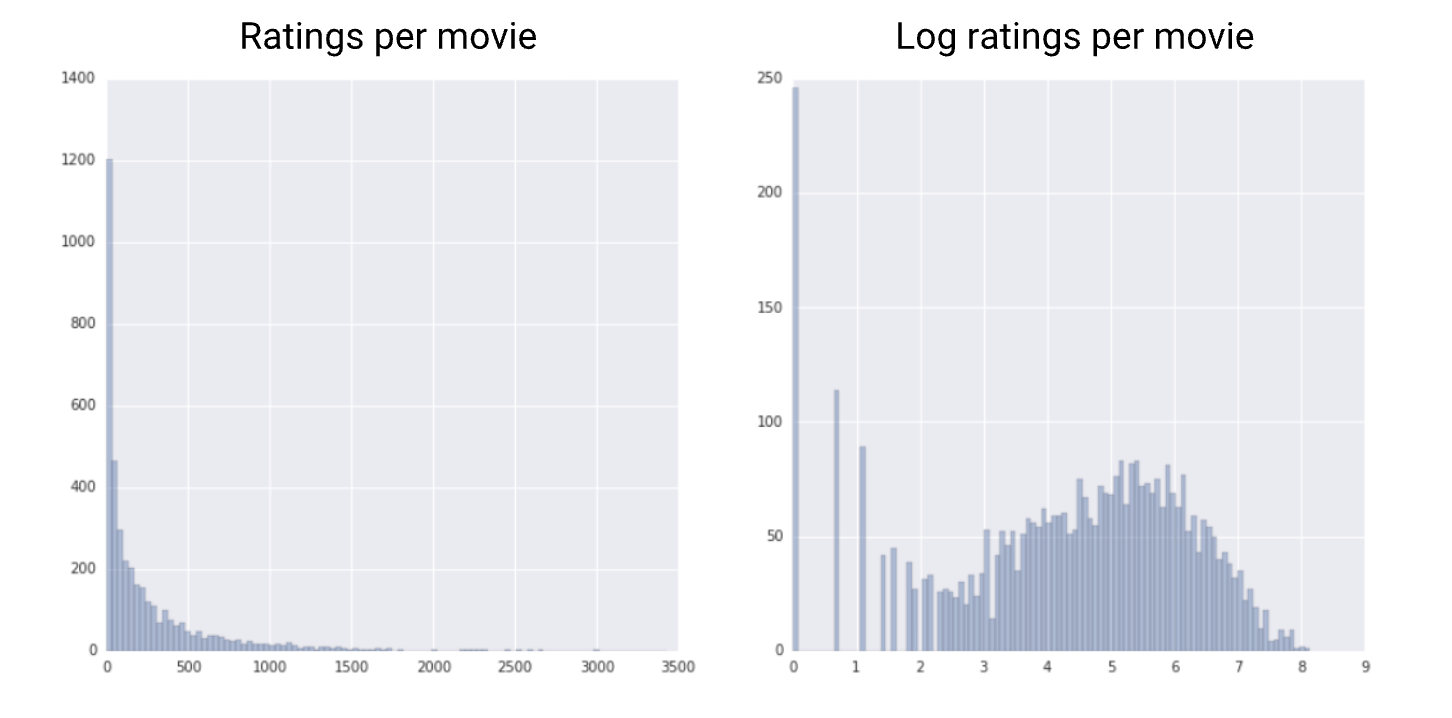
• Another simple clipping strategy is to clip by z-score to ±N𝜎 (for example, limit to ±3𝜎). Note that 𝜎 is the standard deviation.1.2.3. Log Scaling• Log scaling computes the log of your values to compress a wide range to a narrow range.x′=log(x)• Log scaling is helpful when a handful of your values have many points, while most other values have few points. • This data distribution is known as the power law distribution. • Movie ratings are a good example. • In the chart below, most movies have very few ratings (the data in the tail), while a few have lots of ratings (the data in the head). Log scaling changes the distribution, helping to improve linear model performance.
Figure 3:Comparing a raw distribution to its log
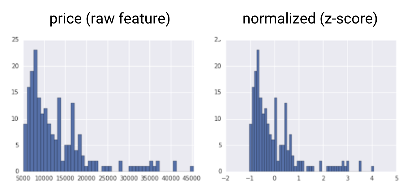
1.2.4. Z-Score• Z-score is a variation of scaling that represents the number of standard deviations away from the mean. • You would use z-score to ensure your feature distributions have mean = 0 and std = 1. • It’s useful when there are a few outliers, but not so extreme that you need clipping.• The formula for calculating the z-score of a point, x, is as follows:x′=(x-𝜇)⁄𝜎• Note:𝜇 is the mean and 𝜎 is the standard deviation.
• Notice that z-score squeezes raw values that have a range of ~ 40000 down into a range from roughly -1 to +4.• Note: Suppose you're not sure whether the outliers truly are extreme. In this case, start with z-score unless you have feature values that you don't want the model to learn; for example, the values are the result of measurement error or a quirk.1.2.5. Summary
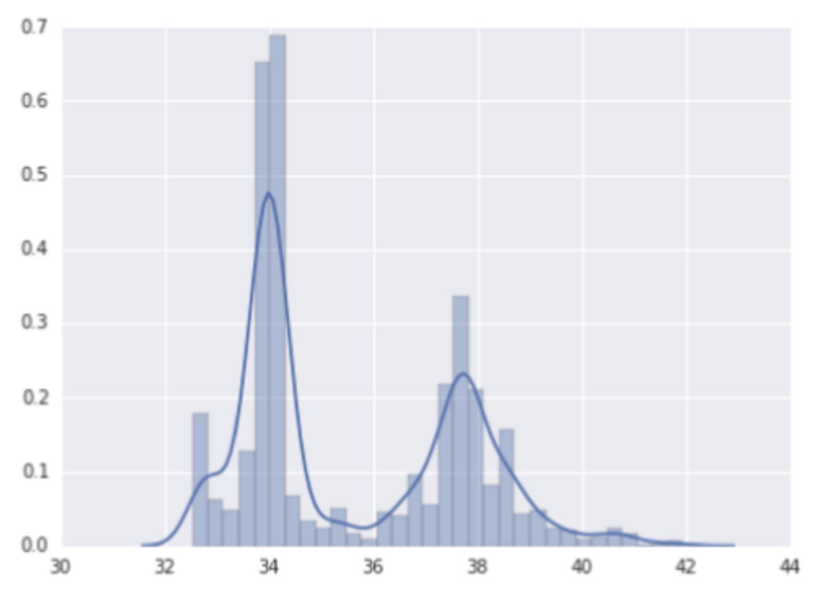
1.3. Bucketing• Look at the distribution in the chart below.
Figure 4:House prices vs. latitude
• Consider ?, If you think latitude might be a good predictor of housing values, should you leave latitude as a floating-point value? Why or why not? (Assume this is a linear model.)– Yes — if latitude is a floating-point value in the dataset, you shouldn't change it.* WRONG: If you feed those floating-point values into your network, it will try to learn a linear relationship between the feature and the label. But a linear relationship isn't likely for latitude. A one-degree increase in latitude (say, from 34 to 35 degrees) may produce some amount of change in the model's output, whereas a different one-degree increase (say, from 35 to 36 degrees) may produce a different amount of change. That's non-linear behavior.–
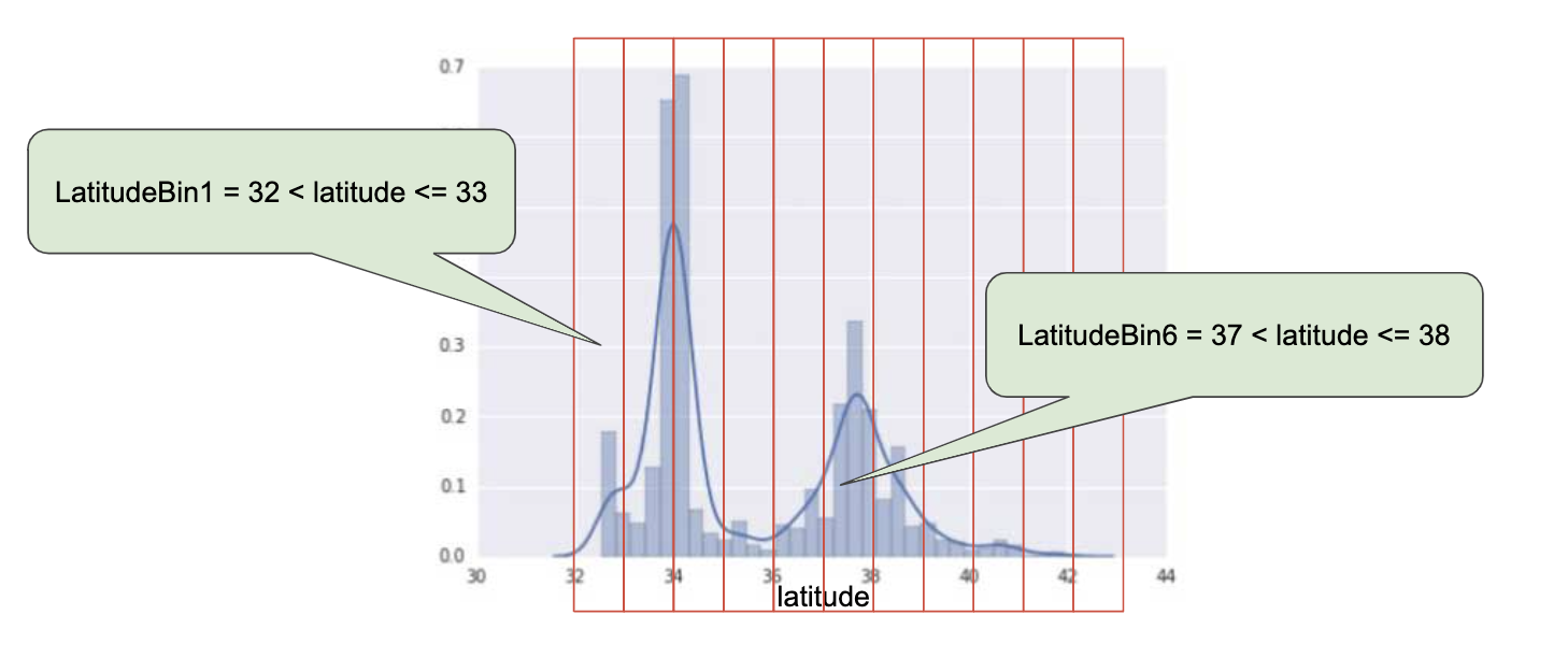
No — there's no linear relationship between latitude and the housing values.* CORRECT: You suspect that individual latitudes and housing values are related, but the relationship is not linear.• • In cases like the latitude example, you need to divide the latitudes into buckets to learn something different about housing values for each bucket. • This transformation of numeric features into categorical features, using a set of thresholds, is called bucketing (or binning). In this bucketing example, the boundaries are equally spaced.
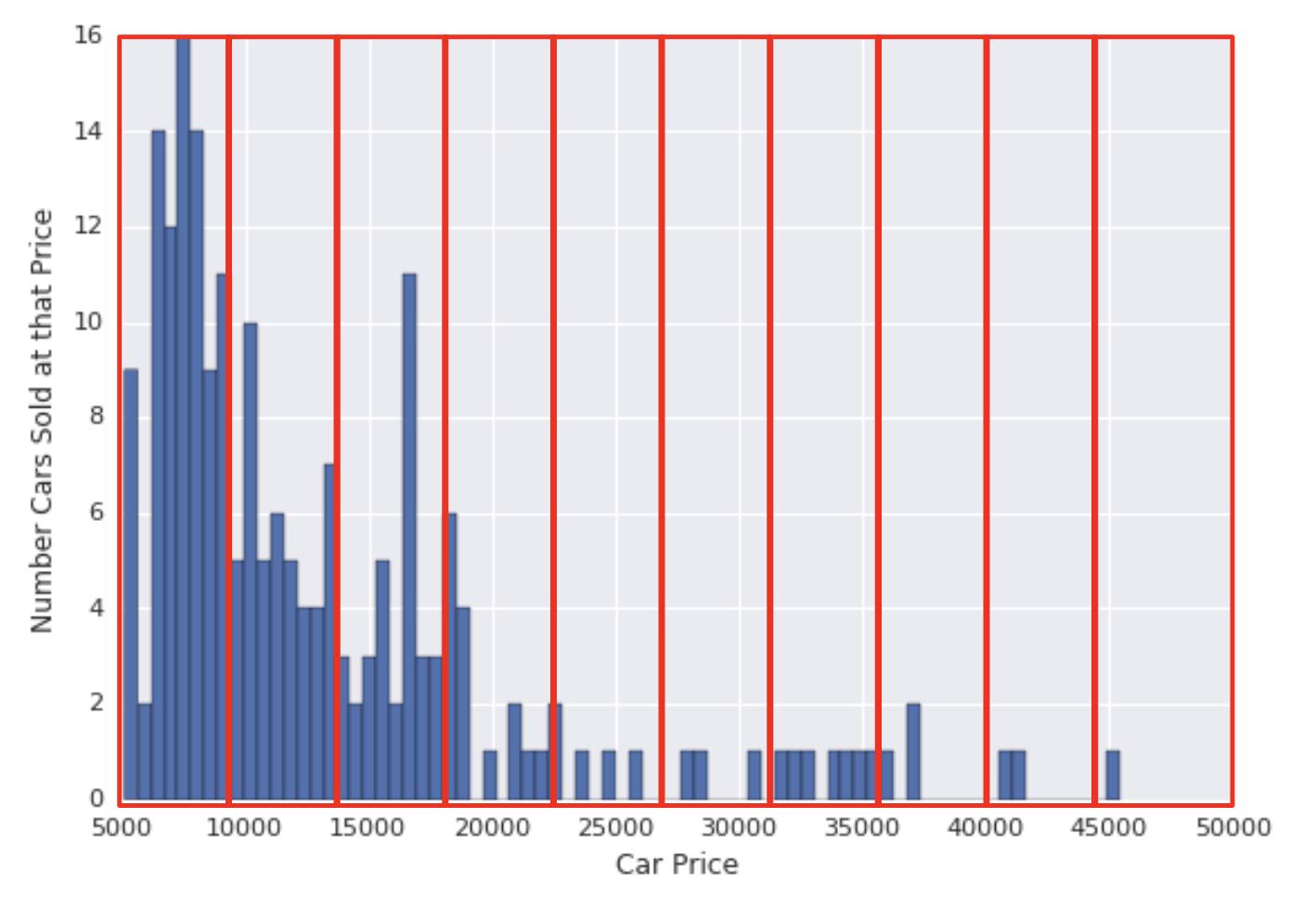
1.3.1. Quantile Bucketing• Let's revisit our car price dataset with buckets added. • With one feature per bucket, the model uses as much capacity for a single example in the >45000 range as for all the examples in the 5000-10000 range. This seems wasteful. How might we improve this situation?
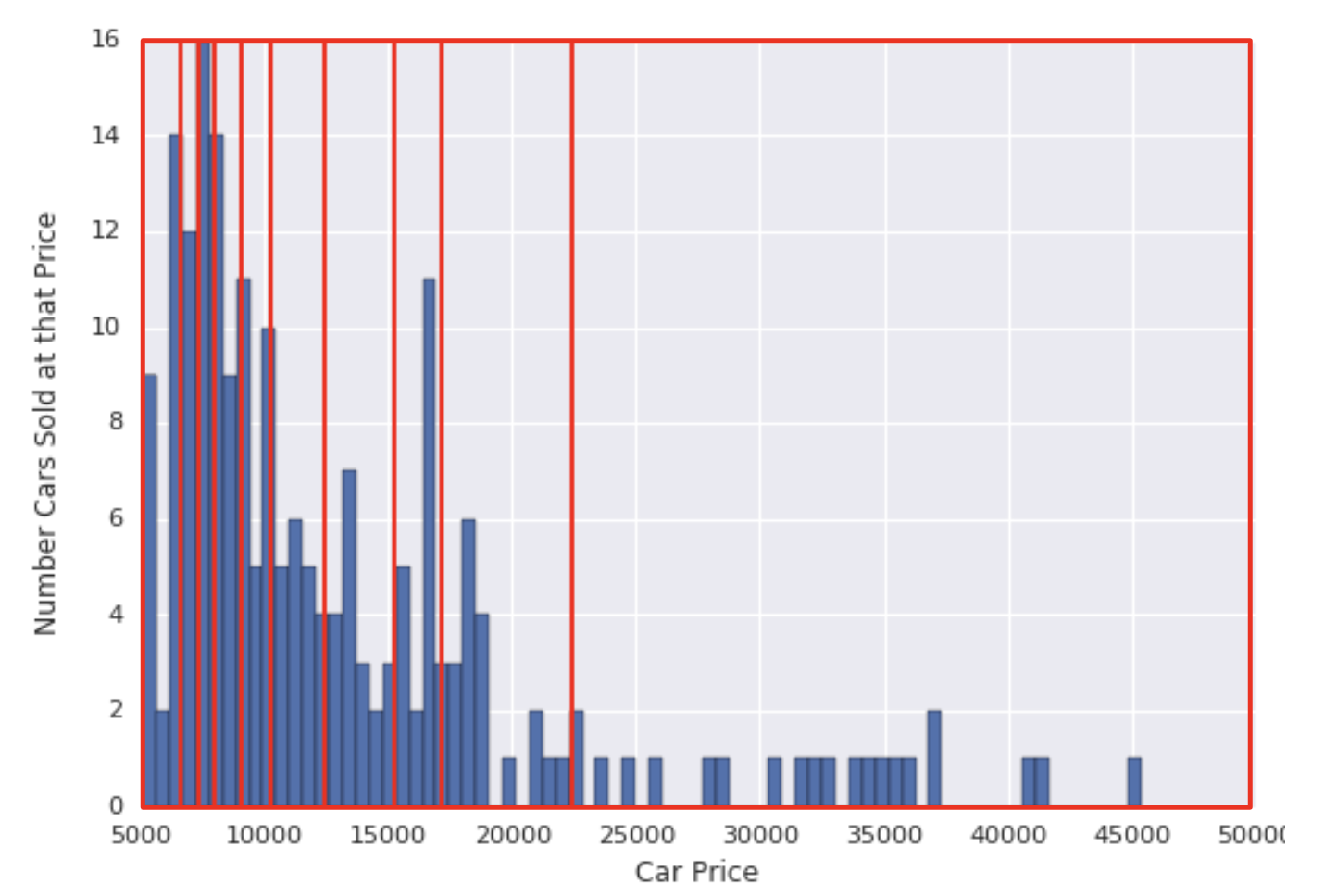
• The problem is that equally spaced buckets don’t capture this distribution well. • The solution lies in creating buckets that each have the same number of points → This technique is called quantile bucketing. – For example, the following figure divides car prices into quantile buckets. – In order to get the same number of examples in each bucket, some of the buckets encompass a narrow price span while others encompass a very wide price span.
1.3.2. Summary• If you choose to bucketize your numerical features, be clear about how you are setting the boundaries and which type of bucketing you’re applying:– Buckets with equally spaced boundaries: the boundaries are fixed and encompass the same range (for example, 0-4 degrees, 5-9 degrees, and 10-14 degrees, or $5,000-$9,999, $10,000-$14,999, and $15,000-$19,999). Some buckets could contain many points, while others could have few or none.– Buckets with quantile boundaries: each bucket has the same number of points. The boundaries are not fixed and could encompass a narrow or wide span of values.