1. Convolutional Neural Networks (CNN)• A breakthrough in building models for image classification came with the discovery that a convolutional neural network (CNN) could be used to progressively extract higher- and higher-level representations of the image content. • To start, the CNN receives an input feature map → a three-dimensional matrix where the size of the first two dimensions corresponds to the length and width of the images in pixels. – The size of the third dimension is 3 (corresponding to the 3 channels of a color image: red, green, and blue). – The CNN comprises a stack of modules, each of which performs three operations.1.1. Convolution• A convolution extracts tiles of the input feature map, and applies filters to them to compute new features, producing an output feature map, or convolved feature (which may have a different size and depth than the input feature map). • • Convolutions are defined by two parameters:– Size of the tiles that are extracted (typically 3x3 or 5x5 pixels).– The depth of the output feature map → the number of filters that are applied.• • During a convolution, the filters (matrices the same size as the tile size) effectively slide over the input feature map's grid horizontally and vertically, one pixel at a time, extracting each corresponding tile (see Figure 1).
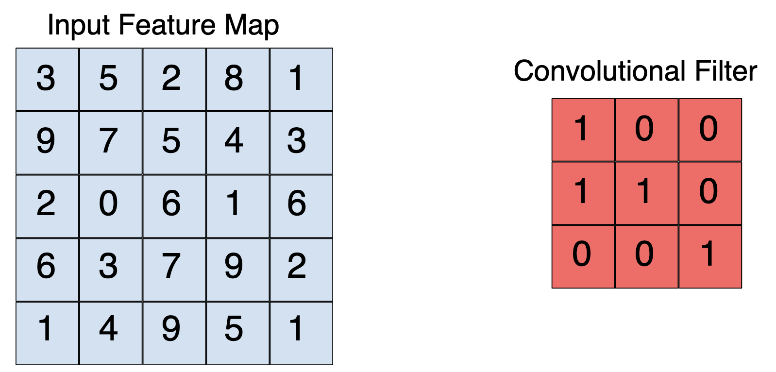
Figure 1:A 3x3 convolution of depth 1 performed over a 5x5 input feature map, also of depth 1. There are nine possible 3x3 locations to extract tiles from the 5x5 feature map, so this convolution produces a 3x3 output feature map.
• Note: In Figure 1, the output feature map (3x3) is smaller than the input feature map (5x5). If you instead want the output feature map to have the same dimensions as the input feature map, you can add padding (blank rows/columns with all-zero values) to each side of the input feature map, producing a 7x7 matrix with 5x5 possible locations to extract a 3x3 tile.• For each filter-tile pair, the CNN performs element-wise multiplication of the filter matrix and the tile matrix, and then sums all the elements of the resulting matrix to get a single value. • Each of these resulting values for every filter-tile pair is then output in the convolved feature matrix (see Figures 2.a and 2.b).
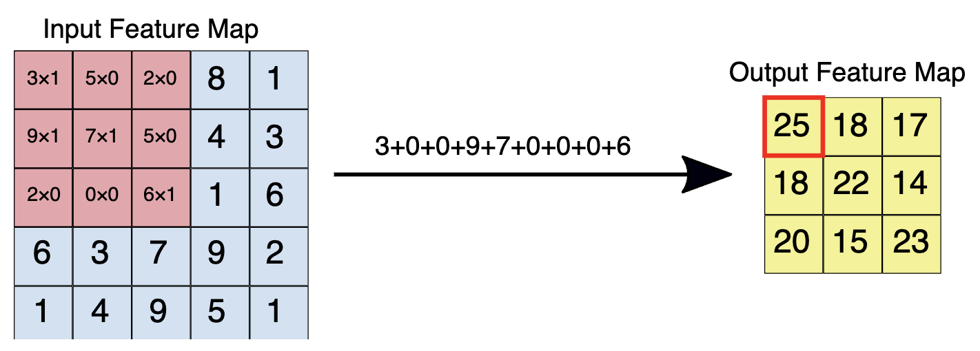
2.a:Left: A 5x5 input feature map (depth 1). Right: a 3x3 convolution (depth 1).
2.b:Left: The 3x3 convolution is performed on the 5x5 input feature map. Right: the resulting convolved feature.
• During training, the CNN "learns" the optimal values for the filter matrices that enable it to extract meaningful features (textures, edges, shapes) from the input feature map. • • As the number of filters (output feature map depth) applied to the input increases, so does the number of features the CNN can extract. – However, the tradeoff is that filters compose the majority of resources expended by the CNN, so training time also increases as more filters are added. – Additionally, each filter added to the network provides less incremental value than the previous one, so engineers aim to construct networks that use the minimum number of filters needed to extract the features necessary for accurate image classification.1.2. ReLU• Following each convolution operation, the CNN applies a Rectified Linear Unit (ReLU) transformation to the convolved feature, in order to introduce nonlinearity into the model. • The ReLU function, F(x)=max(0,x), returns x for all values of x>0, and returns 0 for all values of x⩽0.• ReLU is used as an activation function in a variety of neural networks.1.3. Pooling• After ReLU comes a pooling step, in which the CNN downsamples the convolved feature (to save on processing time), reducing the number of dimensions of the feature map, while still preserving the most critical feature information. • A common algorithm used for this process is called max pooling.• Max pooling operates in a similar fashion to convolution: – We slide over the feature map and extract tiles of a specified size. – For each tile, the maximum value is output to a new feature map, and all other values are discarded. – • Max pooling operations take two parameters:– Size of the max-pooling filter (typically 2x2 pixels)– Stride: the distance, in pixels, separating each extracted tile. * Unlike with convolution, where filters slide over the feature map pixel by pixel, in max pooling, the stride determines the locations where each tile is extracted. * For a 2x2 filter, a stride of 2 specifies that the max pooling operation will extract all nonoverlapping 2x2 tiles from the feature map (see Figure 3).•
Figure 3:Left: Max pooling performed over a 4x4 feature map with a 2x2 filter and stride of 2. Right: the output of the max pooling operation. Note the resulting feature map is now 2x2, preserving only the maximum values from each tile.
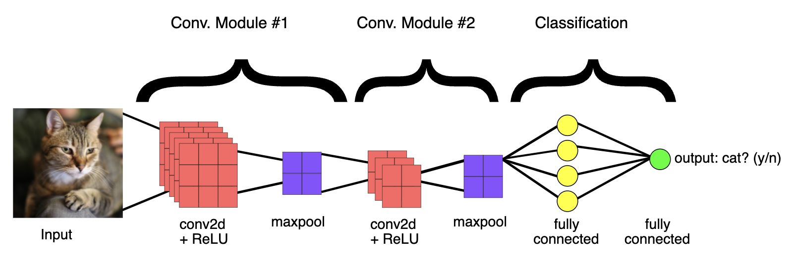
1.4. Fully Connected Layers• At the end of a convolutional neural network are one or more fully connected layers (when two layers are "fully connected," every node in the first layer is connected to every node in the second layer). • Their job is to perform classification based on the features extracted by the convolutions. • Typically, the final fully connected layer contains a softmax activation function, which outputs a probability value from 0 to 1 for each of the classification labels the model is trying to predict.• Figure 4 illustrates the end-to-end structure of a convolutional neural network.
Figure 4:The CNN shown here contains two convolution modules (convolution + ReLU + pooling) for feature extraction, and two fully connected layers for classification. Other CNNs may contain larger or smaller numbers of convolutional modules, and greater or fewer fully connected layers. Engineers often experiment to figure out the configuration that produces the best results for their model.
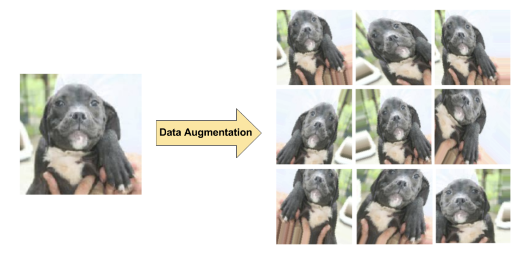
1.5. ExerciseExercise 1: Build a Convnet for Cat vs. Dog ClassificationBack To Top2. Preventing Overfitting• Two techniques to prevent overfitting when building a CNN are:– Data augmentation: artificially boosting the diversity and number of training examples by performing random transformations to existing images to create a set of new variants (see Figure 5). Data augmentation is especially useful when the original training data set is relatively small.– Dropout regularization: Randomly removing units from the neural network during a training gradient step.
Figure 5:Data augmentation on a single dog image (excerpted from the "Dogs vs. Cats" dataset available on Kaggle). Left: Original dog image from training set. Right: Nine new images generated from original image using random transformations.
• Note: Overfitting is more of a concern when working with smaller training data sets. When working with big data sets (e.g., millions of images), applying dropout is unnecessary, and the value of data augmentation is also diminished.2.1. Exercise• Exercise 2: Preventing OverfittingBack To Top3. Leveraging Pretrained Models• Training a convolutional neural network to perform image classification tasks typically requires an extremely large amount of training data, and can be very time-consuming, taking days or even weeks to complete. • But what if you could leverage existing image models trained on enormous datasets, such as via TensorFlow-Slim, and adapt them for use in your own classification tasks?• One common technique for leveraging pretrained models is feature extraction → retrieving intermediate representations produced by the pretrained model, and then feeding these representations into a new model as input. – For example, if you're training an image-classification model to distinguish different types of vegetables, you could feed training images of carrots, celery, and so on, into a pretrained model, and then extract the features from its final convolution layer, which capture all the information the model has learned about the images' higher-level attributes: color, texture, shape, etc. – Then, when building your new classification model, instead of starting with raw pixels, you can use these extracted features as input, and add your fully connected classification layers on top. – To increase performance when using feature extraction with a pretrained model, engineers often fine-tune the weight parameters applied to the extracted features.• • For a more in-depth exploration of feature extraction and fine tuning when using pretrained models, see the following Exercise.4. Next Steps• Federated Learning for Image Classification– More on Federated Learning• Machine Learning is Fun! Part 3: Deep Learning and Convolutional Neural Networks• An Intuitive Explanation of Convolutional Neural Networks• What I learned from competing against a ConvNet on ImageNet• ImageNet Large Scale Visual Recognition Challenge• Learn with Google AIBack To Top