What is Clustering?
When you’re trying to learn about something, say music, one approach might be to look for meaningful groups or collections. You might organize music by genre, while your friend might organize music by decade. How you choose to group items helps you to understand more about them as individual pieces of music. You might find that you have a deep affinity for punk rock and further break down the genre into different approaches or music from different locations. On the other hand, your friend might look at music from the 1980’s and be able to understand how the music across genres at that time was influenced by the sociopolitical climate. In both cases, you and your friend have learned something interesting about music, even though you took different approaches.
In machine learning too, we often group examples as a first step to understand a subject (data set) in a machine learning system. Grouping unlabeled examples is called clustering.
As the examples are unlabeled, clustering relies on unsupervised machine learning. If the examples are labeled, then clustering becomes classification.

Before you can group similar examples, you first need to find similar examples. You can measure similarity between examples by combining the examples’ feature data into a metric, called a similarity measure. When each example is defined by one or two features, it’s easy to measure similarity. For example, you can find similar books by their authors. As the number of features increases, creating a similarity measure becomes more complex. We’ll later see how to create a similarity measure in different scenarios.
What are the Uses of Clustering?
Clustering has a myriad of uses in a variety of industries. Some common applications for clustering include the following:
- market segmentation
- social network analysis
- search result grouping
- medical imaging
- image segmentation
- anomaly detection
After clustering, each cluster is assigned a number called a cluster ID. Now, you can condense the entire feature set for an example into its cluster ID. Representing a complex example by a simple cluster ID makes clustering powerful. Extending the idea, clustering data can simplify large datasets.
For example, you can group items by different features as demonstrated in the following examples:
- Group stars by brightness
- Group organisms by genetic information into a taxonomy.
- Group documents by topic.
Machine learning systems can then use cluster IDs to simplify the processing of large datasets. Thus, clustering’s output serves as feature data for downstream ML systems.
At Google, clustering is used for generalization, data compression, and privacy preservation in products such as YouTube videos, Play apps, and Music tracks.
Generalization
When some examples in a cluster have missing feature data, you can infer the missing data from other examples in the cluster.
- Less popular videos can be clustered with more popular videos to improve recommendations.
Data Compression
As discussed, feature data for all examples in a cluster can be replaced by the relevant cluster ID. This replacement simplifies the feature data and saves storage. These benefits become significant when scaled to large datasets. Further, machine learning systems can use the cluster ID as input instead of the entire feature dataset. Reducing the complexity of input data makes the ML model simpler and faster to train.
Feature data for a single YouTube video can include:
- viewer data on location, time, and demographics
- comment data with timestamps, text, and user IDs
- video tags
Clustering YouTube videos lets you replace this set of features with a
single cluster ID, thus compressing your data.
Privacy Preservation
You can preserve privacy by clustering users, and associating user data with cluster IDs instead of specific users. To ensure you cannot associate the user data with a specific user, the cluster must group a sufficient number of users.
Say you want to add the video history for YouTube users to your model.
Instead of relying on the user ID, you can cluster users and rely on
the cluster ID instead. Now, your model cannot associate the video
history with a specific user but only with a cluster ID that
represents a large group of users.
Clustering Algorithms
Let’s quickly look at types of clustering algorithms and when you should choose each type.
When choosing a clustering algorithm, you should consider whether the algorithm scales to your dataset. Datasets in machine learning can have millions of examples, but not all clustering algorithms scale efficiently. Many clustering algorithms work by computing the similarity between all pairs of examples. This means their runtime increases as the square of the number of examples , denoted as in complexity notation. algorithms are not practical when the number of examples are in millions. This course focuses on the k-means algorithm, which has a complexity of meaning that the algorithm scales linearly with .
Types of Clustering
Several approaches to clustering exist. For an exhaustive list, see A Comprehensive Survey of Clustering Algorithms Xu, D. & Tian, Y. Ann. Data. Sci. (2015) 2: 165. Each approach is best suited to a particular data distribution. Below is a short discussion of four common approaches, focusing on centroid-based clustering using k-means.
Centroid-based Clustering
Centroid-based clustering organizes the data into non-hierarchical clusters, in contrast to hierarchical clustering defined below. k-means is the most widely-used centroid-based clustering algorithm. Centroid-based algorithms are efficient but sensitive to initial conditions and outliers. This course focuses on k-means because it is an efficient, effective, and simple clustering algorithm.

Density-based Clustering
Density-based clustering connects areas of high example density into clusters. This allows for arbitrary-shaped distributions as long as dense areas can be connected. These algorithms have difficulty with data of varying densities and high dimensions. Further, by design, these algorithms do not assign outliers to clusters.

Distribution-based Clustering
This clustering approach assumes data is composed of distributions, such as Gaussian distributions. In Figure 3, the distribution-based algorithm clusters data into three Gaussian distributions. As distance from the distribution’s center increases, the probability that a point belongs to the distribution decreases. The bands show that decrease in probability. When you do not know the type of distribution in your data, you should use a different algorithm.

Hierarchical Clustering
Hierarchical clustering creates a tree of clusters. Hierarchical clustering, not surprisingly, is well suited to hierarchical data, such as taxonomies. See Comparison of 61 Sequenced Escherichia coli Genomes by Oksana Lukjancenko, Trudy Wassenaar & Dave Ussery for an example. In addition, another advantage is that any number of clusters can be chosen by cutting the tree at the right level.

Clustering Workflow
To cluster your data, you’ll follow these steps:
- Prepare data.
- Create similarity metric.
- Run clustering algorithm.
- Interpret results and adjust your clustering.

Prepare Data
As with any ML problem, you must normalize, scale, and transform feature data. While clustering however, you must additionally ensure that the prepared data lets you accurately calculate the similarity between examples. The next sections discuss this consideration.
Create Similarity Metric
Before a clustering algorithm can group data, it needs to know how similar pairs of examples are. You quantify the similarity between examples by creating a similarity metric. Creating a similarity metric requires you to carefully understand your data and how to derive similarity from your features.
Run Clustering Algorithm
A clustering algorithm uses the similarity metric to cluster data. This course focuses on k-means.
Interpret Results and Adjust
Checking the quality of your clustering output is iterative and exploratory because clustering lacks “truth” that can verify the output. You verify the result against expectations at the cluster-level and the example-level. Improving the result requires iteratively experimenting with the previous steps to see how they affect the clustering.
Prepare Data
In clustering, you calculate the similarity between two examples by combining all the feature data for those examples into a numeric value. Combining feature data requires that the data have the same scale. This section looks at normalizing, transforming, and creating quantiles, and discusses why quantiles are the best default choice for transforming any data distribution. Having a default choice lets you transform your data without inspecting the data’s distribution.
Normalizing Data
You can transform data for multiple features to the same scale by normalizing the data. In particular, normalization is well-suited to processing the most common data distribution, the Gaussian distribution. Compared to quantiles, normalization requires significantly less data to calculate. Normalize data by calculating its z-score as follows:
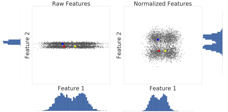
Let’s look at similarity between examples with and without normalization. In Figure 1, you find that red appears to be more similar to blue than yellow. However, the features on the x- and y-axes do not have the same scale. Therefore, the observed similarity might be an artifact of unscaled data. After normalization using z-score, all the features have the same scale. Now, you find that red is actually more similar to yellow. Thus, after normalizing data, you can calculate similarity more accurately.
In summary, apply normalization when either of the following are true:
- Your data has a Gaussian distribution.
- Your data set lacks enough data to create quantiles.
Using the Log Transform
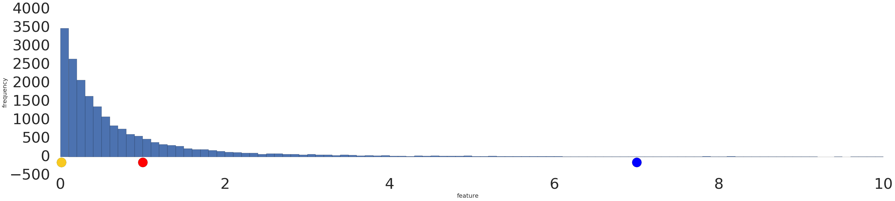
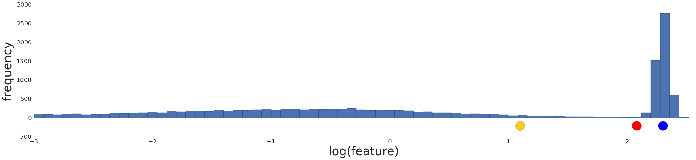
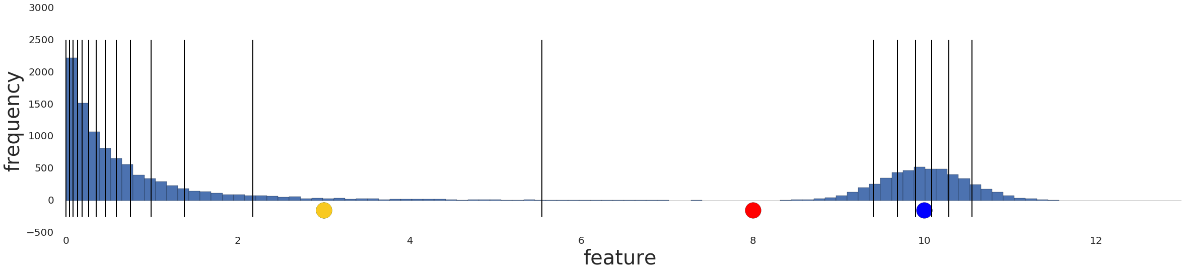
Sometimes, a data set conforms to a power law distribution that clumps data at the low end. In Figure 2, red is closer to yellow than blue.
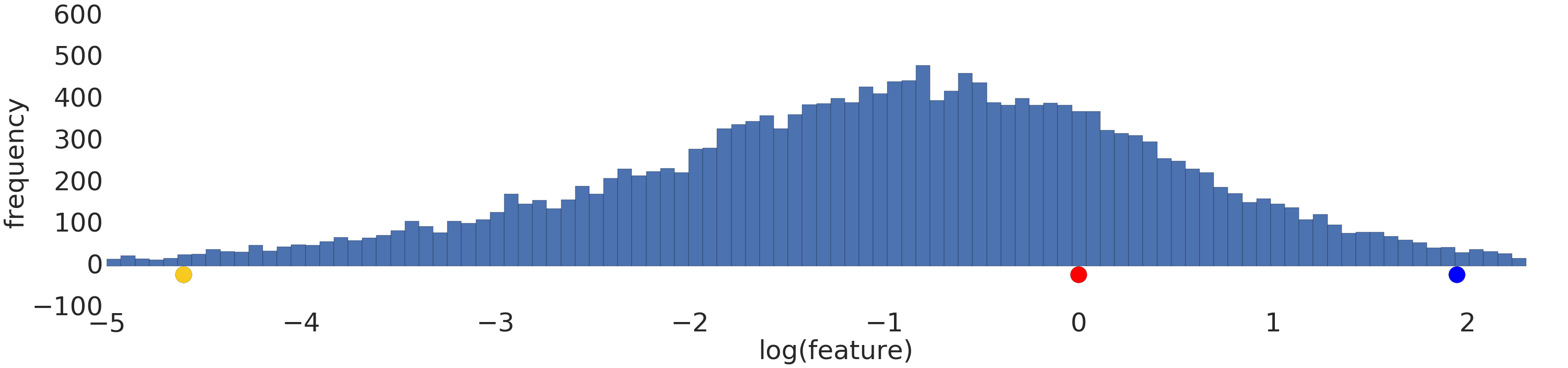
Process a power-law distribution by using a log transform. In Figure 3, the log transform creates a smoother distribution, and red is closer to blue than yellow.
Using Quantiles
Normalization and log transforms address specific data distributions. What if data doesn’t conform to a Gaussian or power-law distribution? Is there a general approach that applies to any data distribution?
Let’s try to preprocess this distribution.
An uncategorizable distribution prior to any preprocessing.
Intuitively, if the two examples have only a few examples between them, then these two examples are similar irrespective of their values. Conversely, if the two examples have many examples between them, then the two examples are less similar. Thus, the similarity between two examples decreases as the number of examples between them increases.
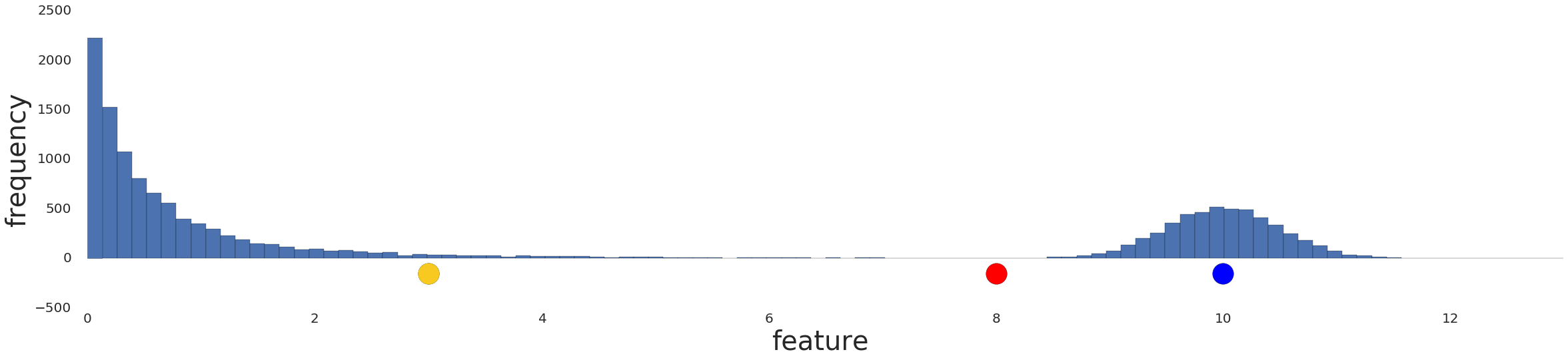
Normalizing the data simply reproduces the data distribution because normalization is a linear transform. Applying a log transform doesn’t reflect your intuition on how similarity works either, as shown in Figure below.
Instead, divide the data into intervals where each interval contains an equal number of examples. These interval boundaries are called quantiles.
Convert your data into quantiles by performing the following steps:
- Decide the number of intervals.
- Define intervals such that each interval has an equal number of examples.
- Replace each example by the index of the interval it falls in.
- Bring the indexes to same range as other feature data by scaling the index values to [0,1].
After converting data to quantiles, the similarity between two examples is inversely proportional to the number of examples between those two examples. Or, mathematically, where “x” is any example in the dataset:
Quantiles are your best default choice to transform data. However, to create quantiles that are reliable indicators of the underlying data distribution, you need a lot of data. As a rule of thumb, to create quantiles, you should have at least examples. If you don’t have enough data, stick to normalization.
Missing Data
If your dataset has examples with missing values for a certain feature but such examples occur rarely, then you can remove these examples. If such examples occur frequently, we have the option to either remove this feature altogether, or to predict the missing values from other examples by using a machine learning model. For example, you can infer missing numerical data by using a regression model trained on existing feature data.
Run the Clustering Algorithm
In machine learning, you sometimes encounter datasets that can have millions of examples. ML algorithms must scale efficiently to these large datasets. However, many clustering algorithms do not scale because they need to compute the similarity between all pairs of points. This means their runtimes increase as the square of the number of points, denoted as . For example, agglomerative or divisive hierarchical clustering algorithms look at all pairs of points and have complexities of and , respectively.
This course focuses on k-means because it scales as , where is the number of clusters. k-means groups points into clusters by minimizing the distances between points and their cluster’s centroid (as seen in Figure below). The centroid of a cluster is the mean of all the points in the cluster.
As shown, k-means finds roughly circular clusters. Conceptually, this means k-means effectively treats data as composed of a number of roughly circular distributions, and tries to find clusters corresponding to these distributions. In reality, data contains outliers and might not fit such a model.
Before running k-means, you must choose the number of clusters, . Initially, start with a guess for . Later, we’ll discuss how to refine this number.
k-Means Clustering Algorithm
To cluster data into clusters, k-means follows the steps below:


k-means Mathematical Proof
Given examples assigned to clusters, minimize the sum of distances of examples to their centroids. Where:
- when the nth example is assigned to the cluster, and 0 otherwise
- is the centroid of cluster
We want to minimize the following expression:
subject to:
and
To minimize the expression with respect to the cluster centroids θk, take the derivative with respect to θk and equate it to 0.
The numerator is the sum of all example-centroid distances in the cluster. The denominator is the number of examples in the cluster. Thus, the cluster centroid is the average of example-centroid distances in the cluster. Hence proved.
Because the centroid positions are initially chosen at random, k-means can return significantly different results on successive runs. To solve this problem, run k-means multiple times and choose the result with the best quality metrics. You’ll need an advanced version of k-means to choose better initial centroid positions.
Interpret Results and Adjusting Clusters
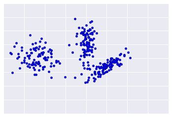
Because clustering is unsupervised, no “truth” is available to verify results. The absence of truth complicates assessing quality. Further, real-world datasets typically do not fall into obvious clusters of examples like the dataset shown in Figure below.
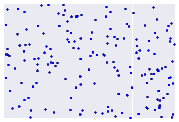
Sadly, real-world data looks more like Figure below, making it difficult to visually assess clustering quality.
The flowchart below summarizes how to check the quality of your clustering. We’ll expand upon the summary in the following sections.

Step One: Quality of Clustering
Checking the quality of clustering is not a rigorous process because clustering lacks “truth”. Here are guidelines that you can iteratively apply to improve the quality of your clustering.
First, perform a visual check that the clusters look as expected, and that examples that you consider similar do appear in the same cluster. Then check these commonly-used metrics as described in the following sections:
- Cluster cardinality
- Cluster magnitude
- Performance of downstream system
Note: While several other metrics exist to evaluate clustering quality, these three metrics are commonly-used and beneficial.
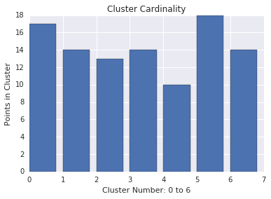
Cluster cardinality
Cluster cardinality is the number of examples per cluster. Plot the cluster cardinality for all clusters and investigate clusters that are major outliers. For example, in Figure below, investigate cluster number 5.
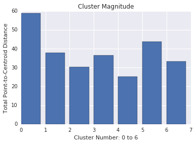
Cluster magnitude
Cluster magnitude is the sum of distances from all examples to the centroid of the cluster. Similar to cardinality, check how the magnitude varies across the clusters, and investigate anomalies. For example, in Figure below, investigate cluster number 0.
Magnitude vs. Cardinality
Notice that a higher cluster cardinality tends to result in a higher cluster magnitude, which intuitively makes sense. Clusters are anomalous when cardinality doesn’t correlate with magnitude relative to the other clusters. Find anomalous clusters by plotting magnitude against cardinality. For example, in Figure below, fitting a line to the cluster metrics shows that cluster number 0 is anomalous.

Performance of Downstream System
Since clustering output is often used in downstream ML systems, check if the downstream system’s performance improves when your clustering process changes. The impact on your downstream performance provides a real-world test for the quality of your clustering. The disadvantage is that this check is complex to perform.
Questions to Investigate If Problems are Found
If you find problems, then check your data preparation and similarity measure, asking yourself the following questions:
- Is your data scaled?
- Is your similarity measure correct?
- Is your algorithm performing semantically meaningful operations on the data?
- Do your algorithm’s assumptions match the data?
Step Two: Performance of the Similarity Measure
Your clustering algorithm is only as good as your similarity measure. Make sure your similarity measure returns sensible results. The simplest check is to identify pairs of examples that are known to be more or less similar than other pairs. Then, calculate the similarity measure for each pair of examples. Ensure that the similarity measure for more similar examples is higher than the similarity measure for less similar examples.
The examples you use to spot check your similarity measure should be representative of the data set. Ensure that your similarity measure holds for all your examples. Careful verification ensures that your similarity measure, whether manual or supervised, is consistent across your dataset. If your similarity measure is inconsistent for some examples, then those examples will not be clustered with similar examples.
If you find examples with inaccurate similarities, then your similarity measure probably does not capture the feature data that distinguishes those examples. Experiment with your similarity measure and determine whether you get more accurate similarities.
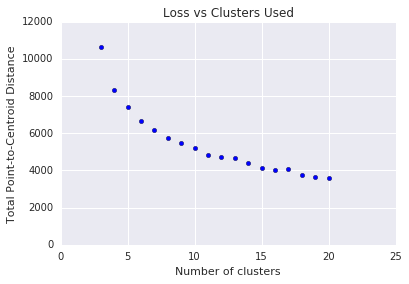
Step Three: Optimum Number of Clusters
k-means requires you to decide the number of clusters beforehand. How do you determine the optimal value of ? Try running the algorithm for increasing and note the sum of cluster magnitudes. As increases, clusters become smaller, and the total distance decreases. Plot this distance against the number of clusters.
As shown in Figure below, at a certain , the reduction in loss becomes marginal with increasing . Mathematically, that’s roughly the where the slope crosses above -1 (). This guideline doesn’t pinpoint an exact value for the optimum but only an approximate value. For the plot shown, the optimum is approximately 11. If you prefer more granular clusters, then you can choose a higher using this plot as guidance.
k-Means Advantages and Disadvantages
Advantages of k-means
- Relatively simple to implement.
- Scales to large data sets.
- Guarantees convergence.
- Can warm-start the positions of centroids.
- Easily adapts to new examples.
- Generalizes to clusters of different shapes and sizes, such as elliptical clusters.
k-means Generalization
What happens when clusters are of different densities and sizes? Look at Figure below. Compare the intuitive clusters on the left side with the clusters actually found by k-means on the right side. The comparison shows how k-means can stumble on certain datasets.

To cluster naturally imbalanced clusters like the ones shown in Figure above, you can adapt (generalize) k-means. In Figure below, the lines show the cluster boundaries after generalizing k-means as:
- Left plot: No generalization, resulting in a non-intuitive cluster boundary.
- Center plot: Allow different cluster widths, resulting in more intuitive clusters of different sizes.
- Right plot: Besides different cluster widths, allow different widths per dimension, resulting in elliptical instead of spherical clusters, improving the result.

While this course doesn’t dive into how to generalize k-means, remember that the ease of modifying k-means is another reason why it’s powerful. For information on generalizing k-means, see Clustering – K-means Gaussian mixture models by Carlos Guestrin from Carnegie Mellon University.
Disadvantages of k-means
Choosing manually.
Use the “Loss vs. Clusters” plot to find the optimal (k), as discussed in Interpret Results.
Being dependent on initial values.
For a low , you can mitigate this dependence by running k-means several times with different initial values and picking the best result. As increases, you need advanced versions of k-means to pick better values of the initial centroids (called k-means seeding). For a full discussion of k- means seeding see, A Comparative Study of Efficient Initialization Methods for the K-Means Clustering Algorithm by M. Emre Celebi, Hassan A. Kingravi, Patricio A. Vela.
Clustering data of varying sizes and density.
k-means has trouble clustering data where clusters are of varying sizes and density. To cluster such data, you need to generalize k-means as described in the Advantages section.
Clustering outliers.
Centroids can be dragged by outliers, or outliers might get their own cluster instead of being ignored. Consider removing or clipping outliers before clustering.
Scaling with number of dimensions.
As the number of dimensions increases, a distance-based similarity measure converges to a constant value between any given examples. Reduce dimensionality either by using PCA on the feature data, or by using “spectral clustering” to modify the clustering algorithm as explained below.
Curse of Dimensionality and Spectral Clustering
These plots show how the ratio of the standard deviation to the mean of distance between examples decreases as the number of dimensions increases. This convergence means k-means becomes less effective at distinguishing between examples. This negative consequence of high-dimensional data is called the curse of dimensionality.

Spectral clustering avoids the curse of dimensionality by adding a pre-clustering step to your algorithm:
- Reduce the dimensionality of feature data by using PCA.
- Project all data points into the lower-dimensional subspace.
- Cluster the data in this subspace by using your chosen algorithm.
Therefore, spectral clustering is not a separate clustering algorithm but a pre-clustering step that you can use with any clustering algorithm. The details of spectral clustering are complicated. See A Tutorial on Spectral Clustering by Ulrike von Luxburg.
Implement k-Means Clustering
Implement k-Means using the TensorFlow k-Means API. The TensorFlow API lets you scale k-means to large datasets by providing the following functionality:
- Clustering using mini-batches instead of the full dataset.
- Choosing more optimal initial clusters using k-means++, which results in faster convergence.
The TensorFlow k-Means API lets you choose either Euclidean distance or cosine distance as your similarity measure.