Source: Probabilistic Machine Learning: An Itroduction by Murphy

Introduction

• A common form of unsupervised learning is dimensionality reduction in which:
  • We learn a mapping from the high-dimensional visible space to a low-dimensional latent space, i.e. $\mathbf{x} \rightarrow \mathbf{z}$ where $\mathbf{z}$ is the embedding.
  • This mapping can be both parametric or nonparametric.
  • The parametric mapping can be used as a preprocessing step for other kinds of learning algorithms.
    • e.g. We might first reduce dimensionality, $\mathbf{x} \rightarrow \mathbf{z}$, and then learn a simple linear classifier on this embedding by mapping $\mathbf{z} \rightarrow y$.

The Importance of Dimensionality Reduction (DR)

1. A lower number of dimensions in data means less training times and fewer computational resources which increases the overall performance of ML algorithms.
2. DR avoids the problem of overfitting.
3. DR takes care of multicollinearity.
4. DR removes noise in data.
5. DR can be used for data compression.

Principal Component Analysis (PCA)

What is PCA?

• The simplest and most widely used form of dimensionality reduction.

• The basic idea is to find a linear and orthogonal project of $\mathbf{x} \rightarrow \mathbf{z}$, such that the $\mathbf{z}$ is a “good approximation” of $\mathbf{x}$.

• In other words, if we project (encode) $\mathbf{x}$ to get $\mathbf{z} = \mathbf{W}^T \mathbf{x}$, and then unproject (decode) $\mathbf{z}$ to get $\hat{\mathbf{x}} = \mathbf{W} \mathbf{z}$, then we want $\hat{\mathbf{x}}$ to be close to $\mathbf{x}$ in $\mathcal{l}_2$ distance.

  • Note: Both encoding and decoding are linear maps.

• This is called reconstruction error or distance. The objective function is to minimize this error.

How to minimize the objective function?

The objective function is to minimize the reconstruction error,

$$\mathcal{L}(\mathbf{W}, \mathbf{Z}) = \frac{1}{N} \sum\limits_{n=1}^N ||\mathbf{x}_n - \mathbf{W} \mathbf{z}_n||^2$$

subject to the constraint that $\mathbf{W}$ is an orthogonal matrix.

Note: If $X$ is a $N \times D$ matrix, and the low-dimensional space has a dimension $L$, then $\mathbf{W}$ size is $L \times D$ and latent factors, $\mathbf{z}$, have the size $N \times L$.

It can be shown that the optimal solution is obtained by setting $\hat{\mathbf{W}} = \mathbf{U}_L$ where $\mathbf{U}_L$ contains the $L$ eigenvectors with largest eigenvalues of the empirical covariance matrix.

$$\hat{\mathbf{\Sigma}} = \frac{1}{N} \sum\limits_{n=1}^N (\mathbf{x}_n - \bar{\mathbf{x}})(\mathbf{x}_n - \bar{\mathbf{x}})^T = \frac{1}{N}\mathbf{X}_c^T \mathbf{X}_c$$

where $\mathbf{X}_c$ is a centered version of $\mathbf{X}$.

Note: Optimal weight vector maximizes the variance of the projected data. In other words, minimizing the reconstruction error is equivalent to maximizing the variance of the projected data. This is why it is often said that PCA finds the directions of maximal variance.

Note: This is equivalent to maximizing the likelihood of a latent linear Gaussian model known as probabilistic PCA.

Note: For details on deriving the optimal solution refer to the book page 653.

Computational Issues

Covariance matrix vs correlation matrix

• So far, we’ve been working with eigendecomposition of the covariance matrix.
• However, it is better to use correlation matrix instead.
• The reason is that otherwise PCA can be “misled” by directions in which the variance is high merely because of the measurement scale.
• Using correlation matrix instead of covariance matrix is equivalent to using standardized data.

Dealing with high-dimensional data

• If $D > N$, it is faster to work with the $N \times N$ matrix $\mathbf{X}\mathbf{X}^T$, instead of the $D \times D$ matrix of $\mathbf{X}^T\mathbf{X}$ as we did previously.
• Let $\mathbf{U}$ be the orthogonal matrix containing eigenvectors of $\mathbf{X}\mathbf{X}^T$ with corresponding eigenvalues in $\mathbf{\Lambda}$. By definition,

$$(\mathbf{X}\mathbf{X}^T)\mathbf{U} = \mathbf{U}\mathbf{\Lambda}$$

• If we pre-multiply by $\mathbf{X}^T$, we get,

$$(\mathbf{X}^T\mathbf{X})(\mathbf{X}^T\mathbf{U}) = (\mathbf{X}^T\mathbf{U})\mathbf{\Lambda}$$

• which means that the eigenvectors of $\mathbf{X}^T\mathbf{X}$ are $\mathbf{V} = \mathbf{X}^T\mathbf{U}$ with eigenvalues $\mathbf{\Lambda}$.
• However, the eigenvectors are not normalized since $||\mathbf{v}_j||^2 = \mathbf{u}_j^T\mathbf{X}\mathbf{X}^T\mathbf{u}_j = \lambda_j\mathbf{u}_j^T\mathbf{u}_j = \lambda_j$.
• The normalized eigenvectors are given by

$$\mathbf{V} = \mathbf{X}^T\mathbf{U}\mathbf{\Lambda}^{\frac{1}{2}}$$

• Note: This method also allows us to use the kernel trick.

Computing PCA using SVD

• Here, we show the equivalence between PCA as computed using eigenvector methods and the truncated SVD.
• Let $\mathbf{U}_\Sigma$ be the top $L$ eigendecomposition of the covariance matrix $\mathbf{\Sigma} \propto \mathbf{X}^T\mathbf{X}$ (we assume $\mathbf{X}$ is normalized).
• Recall that the optimal estimate of the projection weights $\mathbf{W}$ is given by the top $L$ eigenvalues, so $\mathbf{W} = \mathbf{U}_\Sigma$
• Now, from truncated SVD, we have $\mathbf{U}_X\mathbf{S}_X\mathbf{V}_X^T \approx \mathbf{X}$ as the approximation of matrix $\mathbf{X}$.
• We know that the right singular vector of $\mathbf{X}$ are the eigenvectors of $\mathbf{X}^T\mathbf{X}$, so $\mathbf{V}_X = \mathbf{U}_\Sigma = \mathbf{W}$.
• Also, the eigenvalues of the covariance matrix are related to the singular values of the data matrix via $\lambda_k = \frac{\small{s_k^2}}{N}$.
• Suppose we interested in the projected points (also called the principal components or PC scores), rather than the projection matrix,

$$\mathbf{Z} = \mathbf{X}\mathbf{W} = \mathbf{U}_X\mathbf{S}_X\mathbf{V}_X^T\mathbf{V}_X = \mathbf{U}_X\mathbf{S}_X$$

• Finally, if we want to approximately reconstruct the data, we have,

$$\hat{\mathbf{X}} = \mathbf{Z}\mathbf{W}^T = \mathbf{U}_X\mathbf{S}_X\mathbf{V}_X^T$$

• which is precisely the same as a truncated SVD approximation.

• Note: We can perform PCA either using eigendecomposition of $\mathbf{\Sigma}$ or an SVD decomposition of $\mathbf{X}$.

• The SVD is often preferrable for computational reasons.

• For very high-dimensional problems, we can use randomized SVD algorithm.

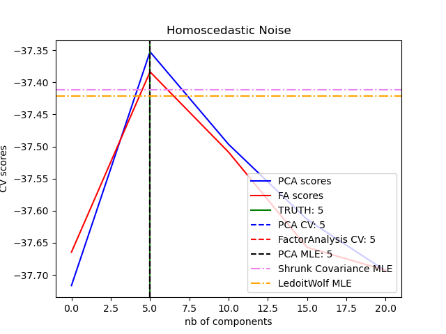
Choosing the number of latent dimensions

• Based on the above we have this: $\hat{\mathbf{x}}_n = \mathbf{W}\mathbf{z}_n + \mathbf{\mu}$ and $\mathbf{z}_n = \mathbf{W}^T (\mathbf{x}_n - \mathbf{\mu})$ where $\mathbf{\mu}$ is the empirical mean.
• If we let $L = \text{rank}(\mathbf{X})$, we get zero reconstruction error.
• To avoid overfitting, it is natural to plot reconstruction error on the test set.
• The problem with PCA is that it is not a proper generative model of data, i.e. if you give it more latent dimensions, it will be able to approximate the test data more accurately.
  • This means that the error continues to go down as the model becomes more complex, unlike the typical supervised learning models where you have a U-shaped curve.
  • A similar problem arises if we plot reconstruction error on the test set using K-means clustering.

Scree plots

• Scree plot $\rightarrow$ A plot of the eigenvalues $\lambda_j$ vs $j$ in order of decreasing magnitude ($j$ is the number of PCs).
• As the number of dimensions (PCs) increases, the eigenvalues get smaller, and so does the reconstruction error.
• A related quantity is the fraction of variance explained, defined as

$$F_L = \frac{\sum_{j=1}^L \lambda_j}{\sum_{j'=1}^{L^{\text{max}}} \lambda_j'}$$

• Note: This captures the same information as the scree plot, but goes up with $L$.
• Note: Similar to using scree plots for clustering, we should look for an “elbow” in the plot.

Importance of Feature Scaling for PCA

Feature scaling through standardization (or Z-score normalization) can be an important preprocessing step for many machine learning algorithms. Standardization involves rescaling the features such that they have the properties of a standard normal distribution with a mean of zero and a standard deviation of one.

While many algorithms (such as SVM, K-nearest neighbors, and logistic regression) require features to be normalized, intuitively we can think of Principle Component Analysis (PCA) as being a prime example of when normalization is important. In PCA we are interested in the components that maximize the variance. If one component (e.g. human height) varies less than another (e.g. weight) because of their respective scales (meters vs. kilos), PCA might determine that the direction of maximal variance more closely corresponds with the ‘weight’ axis, if those features are not scaled. As a change in height of one meter can be considered much more important than the change in weight of one kilogram, this is clearly incorrect.

For a visualized example of the impact of scaling check out this link from sklearn website.

PCA implementation

Source

Exact PCA and the probabilistic interpretation

PCA is used to decompose a multivariate dataset in a set of successive orthogonal components that explain a maximum amount of the variance. In scikit-learn, PCA is implemented as a transformer object that learns $n$ components in its fit method, and can be used on new data to project it on these components.

PCA centers but does not scale the input data for each feature before applying the SVD. The optional parameter whiten=True makes it possible to project the data onto the singular space while scaling each component to unit variance. This is often useful if the models down-stream make strong assumptions on the isotropy of the signal: this is for example the case for Support Vector Machines with the RBF kernel and the K-Means clustering algorithm.

The PCA object also provides a probabilistic interpretation of the PCA that can give a likelihood of data based on the amount of variance it explains. As such it implements a score method that can be used in cross-validation:

Incremental PCA

The PCA object is very useful, but has certain limitations for large datasets. The biggest limitation is that PCA only supports batch processing, which means all of the data to be processed must fit in main memory. The IncrementalPCA object uses a different form of processing and allows for partial computations which almost exactly match the results of PCA while processing the data in a minibatch fashion. IncrementalPCA makes it possible to implement out-of-core Principal Component Analysis either by:

• Using its partial_fit method on chunks of data fetched sequentially from the local hard drive or a network database.
• Calling its fit method on a sparse matrix or a memory mapped file using numpy.memmap.

IncrementalPCA only stores estimates of component and noise variances, in order update explained_variance_ratio_ incrementally. This is why memory usage depends on the number of samples per batch, rather than the number of samples to be processed in the dataset.

As in PCA, IncrementalPCA centers but does not scale the input data for each feature before applying the SVD.

PCA using randomized SVD

It is often interesting to project data to a lower-dimensional space that preserves most of the variance, by dropping the singular vector of components associated with lower singular values.

For instance, if we work with 64x64 pixel gray-level pictures for face recognition, the dimensionality of the data is 4096 and it is slow to train an RBF support vector machine on such wide data. Furthermore we know that the intrinsic dimensionality of the data is much lower than 4096 since all pictures of human faces look somewhat alike. The samples lie on a manifold of much lower dimension (say around 200 for instance). The PCA algorithm can be used to linearly transform the data while both reducing the dimensionality and preserve most of the explained variance at the same time.

The class PCA used with the optional parameter svd_solver='randomized' is very useful in that case: since we are going to drop most of the singular vectors it is much more efficient to limit the computation to an approximated estimate of the singular vectors we will keep to actually perform the transform.

Note: the implementation of inverse_transform in PCA with svd_solver='randomized' is not the exact inverse transform of transform even when whiten=False (default).

SparsePCA & MiniBatchSparsePCA

SparsePCA is a variant of PCA, with the goal of extracting the set of sparse components that best reconstruct the data.

Mini-batch sparse PCA (MiniBatchSparsePCA) is a variant of SparsePCA that is faster but less accurate. The increased speed is reached by iterating over small chunks of the set of features, for a given number of iterations.

Principal component analysis (PCA) has the disadvantage that the components extracted by this method have exclusively dense expressions, i.e. they have non-zero coefficients when expressed as linear combinations of the original variables. This can make interpretation difficult. In many cases, the real underlying components can be more naturally imagined as sparse vectors; for example in face recognition, components might naturally map to parts of faces.

Sparse principal components yields a more parsimonious, interpretable representation, clearly emphasizing which of the original features contribute to the differences between samples.

The following example illustrates 16 components extracted using sparse PCA from the Olivetti faces dataset. It can be seen how the regularization term induces many zeros. Furthermore, the natural structure of the data causes the non-zero coefficients to be vertically adjacent. The model does not enforce this mathematically: each component is a vector $h \in \mathbf{R}^{4096}$, and there is no notion of vertical adjacency except during the human-friendly visualization as 64x64 pixel images. The fact that the components shown below appear local is the effect of the inherent structure of the data, which makes such local patterns minimize reconstruction error. There exist sparsity-inducing norms that take into account adjacency and different kinds of structure; see [Jen09] for a review of such methods. For more details on how to use Sparse PCA, see the Examples section, below.

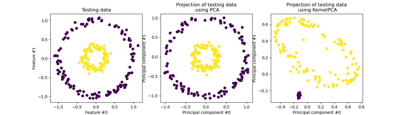
Exact Kernel PCA

KernelPCA is an extension of PCA which achieves non-linear dimensionality reduction through the use of kernels (see Pairwise metrics, Affinities and Kernels) [Scholkopf1997]. It has many applications including denoising, compression and structured prediction (kernel dependency estimation). KernelPCA supports both transform and inverse_transform.

Note: KernelPCA.inverse_transform relies on a kernel ridge to learn the function mapping samples from the PCA basis into the original feature space [Bakir2004]. Thus, the reconstruction obtained with KernelPCA.inverse_transform is an approximation.

Kernel PCA example

Choice of solver for Kernel PCA

While in PCA the number of components is bounded by the number of features, in KernelPCA the number of components is bounded by the number of samples. Many real-world datasets have large number of samples! In these cases finding all the components with a full kPCA is a waste of computation time, as data is mostly described by the first few components (e.g. n_components<=100). In other words, the centered Gram matrix that is eigendecomposed in the Kernel PCA fitting process has an effective rank that is much smaller than its size. This is a situation where approximate eigensolvers can provide speedup with very low precision loss.

The optional parameter eigen_solver='randomized' can be used to significantly reduce the computation time when the number of requested n_components is small compared with the number of samples. It relies on randomized decomposition methods to find an approximate solution in a shorter time.

Truncated SVD & Latent Semantic Analysis

TruncatedSVD implements a variant of singular value decomposition (SVD) that only computes the $k$ largest singular values, where $k$ is a user-specified parameter.

When truncated SVD is applied to term-document matrices (as returned by CountVectorizer or TfidfVectorizer), this transformation is known as latent semantic analysis (LSA), because it transforms such matrices to a “semantic” space of low dimensionality. In particular, LSA is known to combat the effects of synonymy and polysemy (both of which roughly mean there are multiple meanings per word), which cause term-document matrices to be overly sparse and exhibit poor similarity under measures such as cosine similarity.

Mathematically, truncated SVD applied to training samples $\mathbf{X}$ produces a low-rank approximation $\mathbf{X}$:

$$\mathbf{X} \approx \mathbf{X}_k = \mathbf{U}_k\mathbf{\Sigma}_k\mathbf{V}_k^T$$

After this operation, $\mathbf{U}_k\mathbf{\Sigma}_k$ is the transformed training set with $k$ features.

To also transform a test set $\mathbf{X}$, we multiply it with $\mathbf{V}_k$:

$$\mathbf{X}' = \mathbf{X}\mathbf{V}_k$$

Note: Most treatments of LSA in the natural language processing (NLP) and information retrieval (IR) literature swap the axes of the matrix $\mathbf{X}$ so that it has shape n_features $\times$ n_samples. We present LSA in a different way that matches the scikit-learn API better, but the singular values found are the same.

Note: TruncatedSVD is very similar to PCA, but differs in that the matrix X does not need to be centered. When the columnwise (per-feature) means of X are subtracted from the feature values, truncated SVD on the resulting matrix is equivalent to PCA. In practical terms, this means that the TruncatedSVD transformer accepts scipy.sparse matrices without the need to densify them, as densifying may fill up memory even for medium-sized document collections.

Note: While the TruncatedSVD transformer works with any feature matrix, using it on tf–idf matrices is recommended over raw frequency counts in an LSA/document processing setting. In particular, sublinear scaling and inverse document frequency should be turned on (sublinear_tf=True, use_idf=True) to bring the feature values closer to a Gaussian distribution, compensating for LSA’s erroneous assumptions about textual data.

Factor Analysis

I will add the notes on this later.

Autoencoders

• We can think of PCA and FA as learning a linear mapping from $\mathbf{x} \rightarrow \mathbf{z}$, called the encoder, $f_e$, and learning another linear mapping from $\mathbf{z} \rightarrow \mathbf{x}$, called the decoder, $f_d$.
  • The overall reconstruction function has the form: $r(\mathbf{x}) = f_d(f_e(\mathbf{x}))$.
  • The model is trained to minimize: $\mathcal{L}(\mathbf{\theta}) = ||r(\mathbf{x}) - \mathbf{x}||_2^2$.
  • More generally, we can use $\mathcal{L}(\mathbf{\theta}) = - \log{p(\mathbf{x}|r(\mathbf{x}))}$.
• In autoencoder, the encoder and decoder are nonlinear mapping.
• We can think of the hidden units in the middle as a low-dimensional bottleneck between the input and its reconstruction.
• If the hidden layer is wide enough, there is nothing stopping the model from learning the identity function.
  • In order to avoid that degenerate solution, we need to use a narrow bottleneck, i.e. $L \ll D$. This is called undercomplete representation.
  • The other approach is to use $L \gg D$, known as overcomplete representation, but to impose some other kinds of regularization, such as:
    • Adding noise to the inputs
    • Forcing activation units of hidden units to be sparse
    • Imposing a penalty on the derivatives of the hidden units

Bottleneck autoencoders

• We start by considering a special case of a linear autoencoder,
  • It has one hidden layer.
  • The hidden units are cimputed using $\mathbf{z} = \mathbf{W}_1\mathbf{x}$.
  • The output is reconstructed using $\hat{\mathbf{x}} = \mathbf{W}_2\mathbf{z}=\mathbf{W}_2\mathbf{W}_1\mathbf{x} = \mathbf{W}\mathbf{x}$.
  • $\mathbf{W}_1$ is a $L \times D$ matrix, and $\mathbf{W}_2$ is a $D \times L$ matrix, where $L < D$.
  • We train the model to minimize reconstruction error: $\mathcal{L}(\mathbf{W}) = \sum_{n=1}^N ||\mathbf{x}_n - \mathbf{W}\mathbf{x}_n||_2^2$.
  • We can show that $\hat{\mathbf{W}}$ is an orthogonal projection onto the first $L$ eigenvectors of the empirical covariance matrix of the data.
  • Therefore, this is equivalent to PCA.
• If we introduce nonlinearities into the autoencoder, we get a model that is strictly more powerful than PCA. Such methods can learn very useful low dimensional representations of data.
• Nonlinearity can introduced by using MLP, CNN, etc. ( > 1 hidden layer).

Denoising autoencoders (DAE)

• One useful way to control the capacity of an autoencoder is to add noise to its input, and then train the model to reconstruct a clean (uncorrupted) version of the original input $\rightarrow$ denoising autoencoder.
• It can be implemented by adding:
  • Gaussian noise
  • or using Bernoulli dropout

Contractive autoencoders (CAE)

• A different way to regularize autoencoders is by adding this penalty term to the reconstruction loss:

$$\mathbf{\Omega}(\mathbf{z},\mathbf{x})=\lambda||\frac{\partial f_e(\mathbf{x})}{\partial \mathbf{x}}||_F^2 = \lambda \sum ||\Delta_{\mathbf{x}}h_k(\mathbf{x})||_F^2$$

• where $h_k$ is the value of the $k$'th hidden embedding unit.
• Note: We penalize the Frobenius norm of the encoder’s Jacobian.
• Note: A linear operator with Jacobian $\mathbf{J}$ is called contraction if $||\mathbf{J}\mathbf{x}|| \le 1$ for all unit-norm inputs $\mathbf{x}$.
• Note: The Frobenius norm, sometimes also called the Euclidean norm, is matrix norm of an $A_{m \times n}$ matrix and defined as as the square root of the sum of the absolute squares of its elements,
  $$||A||_F = \sqrt{\sum\limits_{i=1}^m \sum\limits_{j=1}^n |a_{i,j}|^2}$$

Variational autoencoders (VAE)

• VAE can be thought of as a probabilistic version of a deterministic autoencoder.
• The principal advantage is that a VAE is a generative model, i.e. it can create new samples, whereas autoencoder just computes embeddings of input vectors.

More on this later.

Spectral Clustering

Take 1

• It is clustering based on the eigenvalue analysis of a pairwise similarity matrix.
• It uses eigenvectors to derive feature vectors for each datapoint.
• The datapoints are then clustered using a feature-based clustering method such as K-means.

Normalized cuts

• We start by creating a weighted undirected graph $\mathbf{W}$, where data vector is a node, and the strength of the $i-j$ edge is a measure of similarity.
  • Note: Typically, we only connect a node to its most similar neighbors to ensure the graph is sparse. This speeds up the computation.
• The goal is to find $K$ clusters of similar points.
  • In other words, we want to find a graph partition into $S_1, S_2, \dots, S_K$ disjoint sets of nodes so as to minimize some kind of cost.
• The objective function, which is called normalized cuts is defined as

$$\text{Ncut}(S_1, S_2, \dots, S_K) \triangleq \frac{1}{2} \sum\limits_{k=1}^{K} \frac{\text{cut}(S_k, \bar{S}_k)}{\text{vol}(S_k)}$$

• where

  • $\text{cut}(S_1, S_2, \dots, S_K) \triangleq \frac{1}{2} \sum\limits_{k=1}^{K} W(S_k, \bar{S}_k)$
  • $W(A,B) \triangleq \sum_{i \in A, j \in B} w_{ij}$
  • $\bar{S}_k = V \backslash S_k$ is the complement of $S_k$, where $V = \{1, \dots, N\}$
  • $\text{vol}(S_k) \triangleq \sum_{i \in A}d_i$
  • $d_i = \sum_{j=1}^N w_{ij}$

• This splits the graph into $K$ clusters with similar nodes in each cluster.

• There’s a method for solving this which is NP-hard.

• A more viable solution is through the eigenvectors of the graph Laplacian.

• The graph Laplacian is defined as $\mathbf{L} \triangleq \mathbf{D} - \mathbf{W}$

  • $\mathbf{W}$ is a symmetric weight matrix for the graph.
  • $\mathbf{D} = \text{diag}(d_i)$ is a diagonal matrix containing the weighted degree of each node, $d_i = \sum_{j} w_{ij}$

• Spectral clustering is very similar to kernel PCA.

Take 2

• A convenient way to represent relationships between data points in a data set is through similarity graphs.
• Vertex (nodes) are the data points.
• Edges’ weight is their similarity.
  • For example, we can use $W_{i,j} = \exp (-d(x_i, x_j)^2 / \sigma^2)$ where $d(.,.)$ is a distance function and $\sigma$ is a parameter.
  • The clustering problem can be formulated as:
    • We want to find a partition of the graph such that the edges between different groups have low weights and the edges within a group have high weights.

Graph Cut

• The simplest way to construct a partition of the graph is to solve the mincut problem, which chooses partitions that minimizes the following objective function

$$\text{cut}(C_1, \dots, C_k) = \sum\limits_{i=1}^{k} \sum\limits_{r \in C_i, s \notin C_i} W_{r,s}$$

• For $k=2$, the mincut problem can be solved efficiently.
  • However, in practice it often does not lead to satisfactory partitions.
    • In many cases, the solution of mincut simply separates one individual vertex from the rest of the graph.
• The simplest solution is to normalize the cut

$$\text{RatioCut}(C_1, \dots, C_k) = \sum\limits_{i=1}^{k} \frac{1}{|C_i|} \sum\limits_{r \in C_i, s \notin C_i} W_{r,s}$$

• It assumes a smaller values if the clusters are not too small.
• Unfortunately, introducing this balancing makes the problem computationally hard to solve.
  • Spectral clustering is a way to relax the problem of minimizing RatioCut.

Graph Laplacian and Relaxed Graph Cuts

• The main mathematical object for spectral clustering is the graph Laplacian matrix.

• The Unnormalized Graph Laplacian is the $m \times m$ matrix $L = D - W$ where $D$ is a diagonal matrix with $D_{i,i} = \sum_{j=1}^m W_{i,j}$.

  • The matrix $D$ is called the degree matrix.

• Note: The following lemma underscores the relationship between RatioCut and the Laplacian matrix.

• LEMMA: Let $C_1, \dots, C_k$ be a clustering and the $H \in \mathbb{R}^{m,k} be the matrix such that$

$$H_{i,j} = \frac{1}{\sqrt{|C_j|}}\mathbb{1}_{[i \in C_j]}$$

• Then, the columns of $H$ are orthonormal to each other and

$$\text{RatioCut}(C_1, \dots, C_k) = \text{trace}(H^TLH)$$

• Note: For the proof, refer to the “Understanding Machine Learning, From Theory to Algorithms, page 316”

• Therefore, to minimize RatioCut we can search for a matrix $H$ whose columns are orthonormal and such that each $H_{i,j}$ is either $0$ or $\frac{1}{\sqrt{|C_j|}}$.

  • Unfortunately, this is integer programming problem which we cannot solve efficiently.

• Instead, we relax the latter requirement and simply search an orthonormal matrix $H \in \mathbb{R}^{m,k}$ that minimizes $\text{trace}(H^TLH)$.

• The solution to this problem is to set $U$ to be the matrix whose columns are the eigenvectors corresponding to the $k$ minimal eigenvalues of $L$.

• The resulting algorithm is called Unnormalized Spectral Clustering.

Spectral Clustering Algorithm

• The spectral clustering algorithm starts with finding the matrix $H$ of the $k$ eigenvectors corresponding to the smallest eigenvalues of the graph Laplacian matrix.
• It then represents points according to the rows of $H$. It is due to the properties of the graph Laplacians that this change of representation is useful.
• In many situations, this change of representation enables the simple k-means algorithm to detect the clusters seamlessly.
• Intuitively, if $H$ is as defined in the Lemma, then each point in the new representation is an indicator vector whose value is nonzero only on the element corresponding to the cluster it belongs to.

Take 3

Source

• Spectral clustering is a technique with roots in graph theory.
• The approach is used to identify communities of nodes in a graph based on the edges connecting them.
• Spectral clustering uses information from the eigenvalues (spectrum) of special matrices built from the graph or the data set.

Eigenvalues and eigenvectors

• Critical to this discussion is the concept of eigenvalues and eigenvectors.
• For a matrix $A$, if there exists a vector $x$ such that $Ax = \lambda x$, then $x$ is called the eigenvector of matrix $A$ with corresponding eigenvalues $\lambda$.
• $x$ only gets scaled (by value of $\lambda$) if multiplied by $A$, instead getting mapped to different place.

import numpy as np

A = np.array([[0,1], [-2,3]])

# find eigenvectors and eigenvalues
vals, vecs = np.linalg.eig(A)

Adjacency Matrix

• We can represent a graph as an adjacency matrix, where the row and column indices represent the nodes, and the entries represen the absense or presence of an edge between the nodes,

A = np.array([
  [0, 1, 1, 0, 0, 0, 0, 0, 1, 1],
  [1, 0, 1, 0, 0, 0, 0, 0, 0, 0],
  [1, 1, 0, 0, 0, 0, 0, 0, 0, 0],
  [0, 0, 0, 0, 1, 1, 0, 0, 0, 0],
  [0, 0, 0, 1, 0, 1, 0, 0, 0, 0],
  [0, 0, 0, 1, 1, 0, 1, 1, 0, 0],
  [0, 0, 0, 0, 0, 1, 0, 1, 0, 0],
  [0, 0, 0, 0, 0, 1, 1, 0, 0, 0],
  [1, 0, 0, 0, 0, 0, 0, 0, 0, 1],
  [1, 0, 0, 0, 0, 0, 0, 0, 1, 0]])

• Note: If the edges were weighted, the weights of the edges would go in this matrix instead of just 1s and 0s.
• Note: Since our graph is undirected, the entries for row i, col j will be equal to the entry at row j, col i.
• Note: The last thing to notice is that the diagonal of this matrix is all 0, since none of our nodes have edges to themselves.

Degree Matrix

• The degree of a node is how many edges connect to it.
  • Note: In a directed graph we could talk about in-degree and out-degree, but in this example we just have degree since the edges go both ways.
  • We could get the degree by taking the sum of the node’s row in the adjacency matrix.
  • The degree matrix is a diagonal matrix where the value at entry (i, i) is the degree of node i.

D = np.diag(A.sum(axis=1))
print(D)

# [[4 0 0 0 0 0 0 0 0 0]
#  [0 2 0 0 0 0 0 0 0 0]
#  [0 0 2 0 0 0 0 0 0 0]
#  [0 0 0 2 0 0 0 0 0 0]
#  [0 0 0 0 2 0 0 0 0 0]
#  [0 0 0 0 0 4 0 0 0 0]
#  [0 0 0 0 0 0 2 0 0 0]
#  [0 0 0 0 0 0 0 2 0 0]
#  [0 0 0 0 0 0 0 0 2 0]
#  [0 0 0 0 0 0 0 0 0 2]]

Graph Laplacian

• Now, let’s calculate the Graph Laplacian.
• Note: The Laplacian is just another matrix representation of a graph.
• It has several beautiful properties, which we will take advantage of for spectral clustering.
• To calculate the normal Laplacian (there are several variants), we just subtract the adjacency matrix from our degree matrix:

L = D-A
print(L)

# [[ 4 -1 -1  0  0  0  0  0 -1 -1]
#  [-1  2 -1  0  0  0  0  0  0  0]
#  [-1 -1  2  0  0  0  0  0  0  0]
#  [ 0  0  0  2 -1 -1  0  0  0  0]
#  [ 0  0  0 -1  2 -1  0  0  0  0]
#  [ 0  0  0 -1 -1  4 -1 -1  0  0]
#  [ 0  0  0  0  0 -1  2 -1  0  0]
#  [ 0  0  0  0  0 -1 -1  2  0  0]
#  [-1  0  0  0  0  0  0  0  2 -1]
#  [-1  0  0  0  0  0  0  0 -1  2]]

• Note: The Laplacian’s diagonal is the degree of our nodes, and the off diagonal is the negative edge weights. This is the representation we are after for performing spectral clustering.

Eigenvalues of Graph Laplacian

• As mentioned, the Laplacian has some beautiful properties. To get a sense for this, let’s examine the eigenvalues associated with the Laplacian as I add edges to our graph:

• We see that when the graph is completely disconnected, all ten of our eigenvalues are 0.
• As we add edges, some of our eigenvalues increase. In fact, the number of 0 eigenvalues corresponds to the number of connected components in our graph!
• Look closely as that final edge is added, connecting the two components into one. When this happens, all of the eigenvalues but one have been lifted:

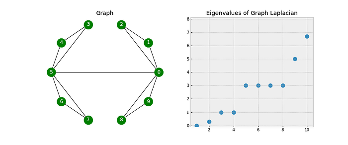
• Note: The first eigenvalue is 0 because we only have one connected component (the whole graph is connected).
• The corresponding eigenvector will always have constant values (in this example all the values are close to 0.32).
• The first nonzero eigenvalue is called the spectral gap. The spectral gap gives us some notion of the density of the graph. If this graph was densely connected (all pairs of the 10 nodes had an edge), then the spectral gap would be 10.
• The second eigenvalue is called the Fiedler value, and the corresponding vector is the Fiedler vector.
  • The Fiedler value approximates the minimum graph cut needed to separate the graph into two connected components.
• Recall, that if our graph was already two connected components, then the Fiedler value would be 0.
• Each value in the Fiedler vector gives us information about which side of the cut that node belongs.
• Let’s color the nodes based on whether their entry in the Fielder vector is positive or not:

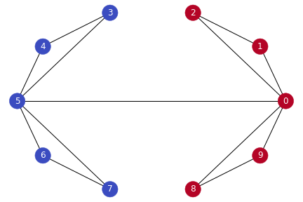
• This simple trick has segmented our graph into two clusters! Why does this work?

• Remember that zero eigenvalues represent connected components.

• Eigenvalues near zero are telling us that there is almost a separation of two components.

• Here we have a single edge, that if it didn’t exist, we’d have two separate components. So the second eigenvalue is small.

• Summary so far:

  • The first eigenvalue is 0 because we have one connected component.
  • The second eigenvalue is near 0 because we’re one edge away from having two connected components.
  • We also saw that the vector associated with that value tells us how to separate the nodes into those approximately connected components.

---

• You may have noticed that the next two eigenvalues are also pretty small. That tells us that we are “close” to having four separate connected components.
  • In general, we often look for the first large gap between eigenvalues in order to find the number of clusters expressed in our data. See the gap between eigenvalues four and five?
• Having four eigenvalues before the gap indicates that there is likely four clusters.
• ==The vectors associated with the first three positive eigenvalues should give us information about which three cuts need to be made in the graph to assign each node to one of the four approximated components. ==
• Let’s build a matrix from these three vectors and perform K-Means clustering to determine the assignments:

from sklearn.cluster import KMeans

# our adjacency matrix
print("Adjacency Matrix:")
print(A)

# Adjacency Matrix:
# [[0. 1. 1. 0. 0. 1. 0. 0. 1. 1.]
#  [1. 0. 1. 0. 0. 0. 0. 0. 0. 0.]
#  [1. 1. 0. 0. 0. 0. 0. 0. 0. 0.]
#  [0. 0. 0. 0. 1. 1. 0. 0. 0. 0.]
#  [0. 0. 0. 1. 0. 1. 0. 0. 0. 0.]
#  [1. 0. 0. 1. 1. 0. 1. 1. 0. 0.]
#  [0. 0. 0. 0. 0. 1. 0. 1. 0. 0.]
#  [0. 0. 0. 0. 0. 1. 1. 0. 0. 0.]
#  [1. 0. 0. 0. 0. 0. 0. 0. 0. 1.]
#  [1. 0. 0. 0. 0. 0. 0. 0. 1. 0.]]

# diagonal matrix
D = np.diag(A.sum(axis=1))

# graph laplacian
L = D-A

# eigenvalues and eigenvectors
vals, vecs = np.linalg.eig(L)

# sort these based on the eigenvalues
vecs = vecs[:,np.argsort(vals)]
vals = vals[np.argsort(vals)]

# kmeans on first three vectors with nonzero eigenvalues
kmeans = KMeans(n_clusters=4)
kmeans.fit(vecs[:,1:4])
colors = kmeans.labels_

print("Clusters:", colors)

# Clusters: [2 1 1 0 0 0 3 3 2 2]

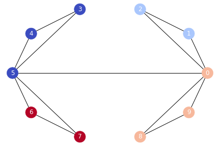
Summary: We first took our graph and built an adjacency matrix. We then created the Graph Laplacian by subtracting the adjacency matrix from the degree matrix. The eigenvalues of the Laplacian indicated that there were four clusters. The vectors associated with those eigenvalues contain information on how to segment the nodes. Finally, we performed K-Means on those vectors in order to get the labels for the nodes. Next, we’ll see how to do this for arbitrary data.

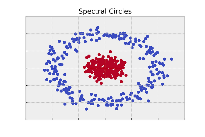
Spectral Clustering Arbitrary Data

• The points are drawn from two concentric circles with some noise added.

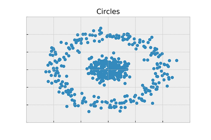
• This data isn’t in the form of a graph. So first, let’s just try a cookie cutter algorithm like K-Means. K-Means will find two centroids and label the points based on which centroid they are closest too.

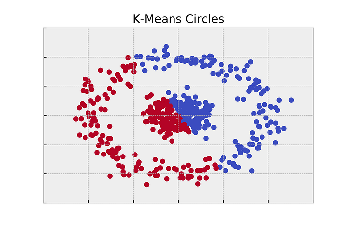
• Obviously, K-Means wasn’t going to work. It operates on euclidean distance, and it assumes that the clusters are roughly spherical. This data (and often real world data) breaks these assumptions.

Nearest Neighbor Graph

• There are a couple of ways to treat our data as a graph. The easiest way is to construct a k-nearest neighbors graph.
  • A k-nearest neighbors graph treats every data point as a node in a graph.
  • An edge is then drawn from each node to its $k$ nearest neighbors in the original space.
  • Generally, the algorithm isn’t too sensitive of the choice of $k$. Smaller numbers like 5 or 10 usually work pretty well.
• Look at the picture of the data again, and imagine that each point is connected to its 5 closest neighbors.
  • Any point in the outer ring should be able to follow a path along the ring, but there won’t be any paths into the inner circle.
  • It’s pretty easy to see that this graph will have two connected components: the outer ring and the inner circle.
• Since we’re only separating this data into two components, we should be able to use our Fiedler vector trick from before.
• Here’s the code I used to perform spectral clustering on this data:

from sklearn.datasets import make_circles
from sklearn.neighbors import kneighbors_graph
import numpy as np

# create the data
X, labels = make_circles(n_samples=500, noise=0.1, factor=.2)

# use the nearest neighbor graph as our adjacency matrix
A = kneighbors_graph(X, n_neighbors=5).toarray()
print(A)

# [[0. 0. 0. ... 0. 0. 0.]
#  [0. 0. 0. ... 0. 0. 0.]
#  [0. 0. 0. ... 0. 0. 0.]
#  ...
#  [0. 0. 0. ... 0. 1. 0.]
#  [0. 0. 0. ... 0. 0. 0.]
#  [0. 0. 0. ... 0. 0. 0.]]
 
# create the graph laplacian
D = np.diag(A.sum(axis=1))
L = D-A

# find the eigenvalues and eigenvectors
vals, vecs = np.linalg.eig(L)

# sort
vecs = vecs[:,np.argsort(vals)]
vals = vals[np.argsort(vals)]

# use Fiedler value to find best cut to separate data
clusters = vecs[:,1] > 0

Other Approaches

• The nearest neighbor graph is a nice approach, but it relies on the fact that “close” points should belong in the same cluster.

• Depending on your data, that might not be true.

• A more general approach is to construct an affinity matrix.

• An affinity matrix is just like an adjacency matrix, except the value for a pair of points expresses how similar those points are to each other.

• If pairs of points are very dissimilar then the affinity should be 0. If the points are identical, then the affinity might be 1.

• In this way, the affinity acts like the weights for the edges on our graph.

• How to decide on what it means for two data points to be similar is one of the most important questions in machine learning.

  • Often domain knowledge is the best way to construct a similarity measure. If you have access to domain experts, ask them this question.

• There are also entire fields dedicated to learning how to construct similarity metrics directly from data.

  • For example, if you have some labeled data, you can train a classifier to predict whether two inputs are similar or not based on if they have the same label. This classifier can then be used to assign affinity to pairs of unlabeled points.

Conclusion

• Spectral clustering is a flexible approach for finding clusters when your data doesn’t meet the requirements of other common algorithms.
• First, we formed a graph between our data points. The edges of the graph capture the similarities between the points.
• The eigenvalues of the Graph Laplacian can then be used to find the best number of clusters, and the eigenvectors can be used to find the actual cluster labels.

Take 4

Another nice article comparing Kernel K-means with spectral clustering.

Other resources

• A Tutorial on Spectral Clustering, U. Luxburg, March 2007
• Comparing different clustering algorithms