aMath of Gradient Boosting Table of Content1. Introduction 2. Bagging 2.1. Bagging vs. Boosting 3. Gradient Boosting 3.1. The Idea of Additive Modeling 3.2. Gradient Boosting Algorithm 3.3. Pseudo-Residuals 4. How the Algorithm Works 4.1. Notations 4.2. STEP 1: Initialize the Model with a Constant Value 4.3. STEP 2 4.3.1. STEP 2.1: Compute Pseudo-Residuals 4.3.2. STEP 2.2: Fit Base Learners on the Pseudo-Residuals 4.3.3. STEP 2.3: Find the Optimum 𝛾$𝛾$ 4.3.4. STEP 2.4: Model Update 4.4. STEP 3 4.4.1. Why the name ‘Gradient Boosting’?

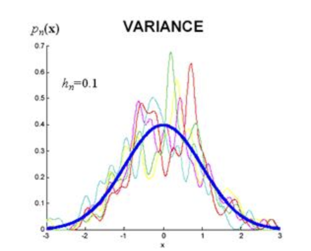
Source 1. Introduction• Boosting is an ensemble learning technique. • Conceptually, these techniques involve: – 1. learning base learners; – 2. using all of the models to come to a final prediction. – • Ensemble learning techniques are of different types and all differ from each other in terms of how they go about implementing the learning process for the base learners and then using their output to give out the final result. • • Techniques that are used in ensemble learning are Bootstrap Aggregation (a.k.a. Bagging), Boosting, Cascading models and Stacked Ensemble Models. • Gradient Boosting is a generic model which works with any loss function which is differentiable, however, seeing it work with a squared loss model alone does not completely explain what it does during the learning process. 2. Bagging• Bagging is a combination of two subsequent steps:1. Bootstrap sampling of the dataset, into M${\displaystyle M}$ subsets. Each one of these M${\displaystyle M}$ subsets are then used to learn a model. These models are called as base learners/models.2. Taking a majority vote to declare the final prediction value. • Since in bagging, a subset of the dataset is used to train a base model, each of the base learners is likely to overfit (since each model has lesser examples to learn from, they may not generalize well). • Taking majority vote is gives a model that has a variance which is the average of the variances of all base learners (Figure 1).

Figure 1:Blue curve represents the variance of the final model, all other curves are variances of the base learners

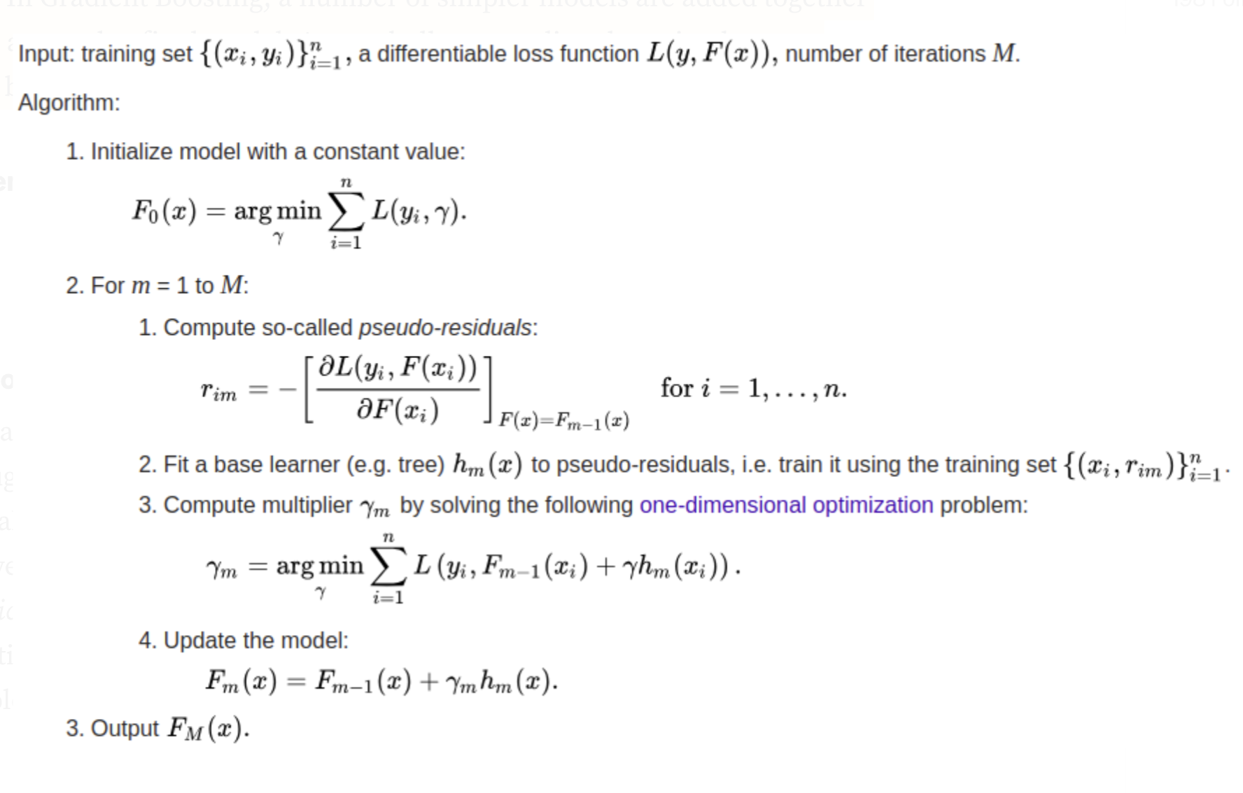
2.1. Bagging vs. Boosting• Boosting is quite different from Bagging in its approach of training base learners and using them to give final results. • Bagging learns base learners from independently bootstrapped subsets of data, and hence we can train all the base learners simultaneously in a parallel environment.• Boosting, on the other hand, trains the base learners sequentially - models are trained one after the other. – Therefore, training base learners in parallel is impossible. – Moreover, in a Boosting algorithm we start with a high bias model. – The actual model is first initialized with a constant value. – It is then progressively made less biased by adding base learners to it. – We shall see how Gradient Boosting goes about learning a final model that has a much lower bias given an appropriate number of base learners. 3. Gradient Boosting3.1. The Idea of Additive Modeling• Additive modeling is at the foundation of Boosting algorithms. • The idea is simple:– Form a complex function by adding together a bunch of simpler terms. • In Gradient Boosting, a number of simpler models are added together to give a complex final model. As we shall see, gradient boosting learns a model by taking a weighted sum of a suitable number of base learners. 3.2. Gradient Boosting Algorithm

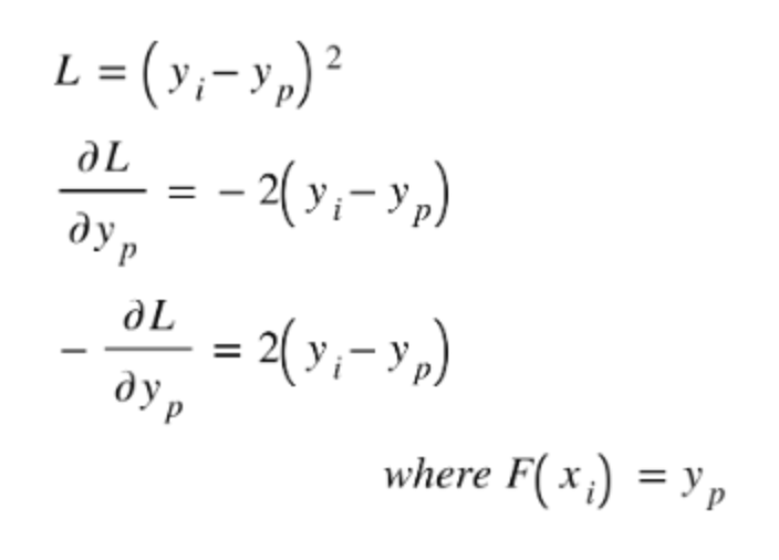
3.3. Pseudo-Residuals• In the algorithm, step 2(1) mentions about computing ‘pseudo-residuals’. • Although there is hardly any concrete conceptual definition of what a pseudo-residual is, but mathematically what is mentioned is how you define it. • However, I feel the name is kind of borrowed from the difference (yactual-ypredicted${\displaystyle y_{\text{actual}}-y_{\text{predicted}}}$) which is often referred to as residual error which we get by taking a derivative of square loss function L${\displaystyle L}$ w.r.t. the predicted value F(xi)${\displaystyle F(x_i)}$ for i${\displaystyle i}$th example.

• Probably no loss function differentiates to give residual, yet, in the case of squared loss, its differentiation gives a function that is closest to the residual error ‘visually’. • May be the name has been borrowed from this. • Nonetheless, gradient boosting has nothing to do with the derivative of loss function w.r.t. hypothesis being equal to the residual error. 4. How the Algorithm Works• We may have got an idea of one of the things we do in gradient boosting - taking derivatives of the loss function w.r.t. the hypothesis function. • Needless to say, the loss function has to be differentiable w.r.t. the hypothesis function. • As the algorithm says, gradient boosting takes the training set and a loss function as inputs. 4.1. Notations• Some of the notations used in the algorithm taken from Wikipedia (posted above) are somewhat inconsistent. So, I shall use my own notations for those variables.• FM(x)${\displaystyle F_M(x)}$ → Final model that will be learned by taking weighted sum of M${\displaystyle M}$ base learners (additive modeling).• Fm(x)${\displaystyle F_m(x)}$ → Model obtained by adding m={1,2,…,m}${\displaystyle m=\{1,2,\dots ,m\}}$ base learners and the initial constant value of FM(x)${\displaystyle F_M(x)}$. 4.2. STEP 1: Initialize the Model with a Constant Value• We find a constant model F0=𝛾${\displaystyle F_0=𝛾}$ that fits to the actual y${\displaystyle y}$-values. • Why a constant model? – This is where the idea of boosting starts to manifest - going from a high bias to a low bias model. – We start with a constant function (no other function can have more bias than a constant function, unless the dataset is so boring that even a constant model fits it)– Then go on through a number of steps finding a function that has a reasonably low bias. – In some texts, you may find initializing the model with 0 (zero). * That is also a constant function, but quite possibly we can start with a slightly better option. * Let’s say the initial model is a constant function 𝛾${\displaystyle 𝛾}$. The loss function for a constant function then is as follows:(1)n∑i=1L(yi,𝛾)$$\sum _{i=1}^{n}L(y_i,𝛾)$$• Therefore, 𝛾optimal${\displaystyle {𝛾}_{\text{optimal}}}$ is determined by the solving following optimization problem: (2)F0(x)=𝛾optimal=min𝛾n∑i=1L(yi,𝛾)$$F_0(x)={𝛾}_{\text{optimal}}={\min }_{𝛾}\sum _{i=1}^{n}L(y_i,𝛾)$$ • This is for sure better than a model initialized with zero. – Particularly for squared loss error, F0(x)${\displaystyle F_0(x)}$ is equal to the mean of the actual y${\displaystyle y}$-values, i.e., F0(x)=ymean${\displaystyle F_0(x)=y_{\text{mean}}}$ when squared loss is used.• Often in texts, this model is not counted as one of the base learners although the final model is going to be an additive model obtained from base learners and this model will also be one of addends. • There is one difference though - all the models that are called as base learners in the literature, are fitted on the pseudo-residuals and not on the y${\displaystyle y}$-values of the actual dataset (we shall see how it is done in step 2). • Since F0(x)${\displaystyle F_0(x)}$ is fitted on the y${\displaystyle y}$-values, probably that is why it is not considered as one of the base learners in the literature.• At this point FM(x)=F0(x).FM(x)${\displaystyle F_M(x)=F_0(x).F_M(x)}$, however, is subject to updates until all the M${\displaystyle M}$ base learners are added to it with suitable weights. 4.3. STEP 2• This step is to be followed for each base learner from m=1${\displaystyle m=1}$ to m=M${\displaystyle m=M}$. Note that gradient boosting adds one model at a time, one after the other.• Gradient boosting algorithm has to be configured with a suitable value of hyperparameter M${\displaystyle M}$ (number of base learners) prior to execution. 4.3.1. STEP 2.1: Compute Pseudo-Residuals• Pseudo-residuals are computed for each i${\displaystyle i}$th training example: (3)rim=𝜕L(y, Fm-1(x))

𝜕Fm-1(x)|x=xi,y=yi ∀i∈{1,2,…,n}$$r_{im}=\frac{𝜕L(y,F_{m-1}(x))}{𝜕F_{m-1}(x)}{|}_{x=x_i,y=y_i}\forall i\in \{1,2,\dots ,n\}$$ • Note that Fm-1(x)${\displaystyle F_{m-1}(x)}$ is the model obtained by adding m-1${\displaystyle m-1}$ weighted base learners and the initial constant function. • The m${\displaystyle m}$th base learner has not yet been added. • Each residual calculation rim${\displaystyle r_{im}}$ for i${\displaystyle i}$th training example corresponding to the current base learner m${\displaystyle m}$ (which will be trained and added in step 2.2) is done on the weighted sum of base learners from 1 to m-1${\displaystyle m-1}$ and the initial constant function (step 1). • Recall that after step 1, F0(x)=𝛾${\displaystyle F_0(x)=𝛾}$ does not include any term corresponding to any base learner – Recall that F0(x)${\displaystyle F_0(x)}$ is most often not called as a base learner in the literature. It is treated only as an initial value of the model. 4.3.2. STEP 2.2: Fit Base Learners on the Pseudo-Residuals• For this step, a new dataset is derived from the given dataset. The dataset Dmodified${\displaystyle D_{\text{modified}}}$ is defined as shown in equation (4): (4)Dmodified={(xi,rim): i=1,2,…,n}$$D_{\text{modified}}=\{(x_i,r_{im}):i=1,2,\dots ,n\}$$ • A base learner hm(x)${\displaystyle h_m(x)}$ is trained and fitted on this dataset.• At this point, we have everything required to determine Fm(x)${\displaystyle F_m(x)}$. We do it as following: (5)Fm(x)=Fm-1(x)+𝛾hm(x)$$F_m(x)=F_{m-1}(x)+𝛾h_m(x)$$ • Why does doing this make sense?– It is straightforward to see why this equation makes sense if we compare it with weight updates done in Gradient Descent (equation (6)). – Weights in gradient descent are moved in the direction in which loss L${\displaystyle L}$ decreases. – How much the weights should be moved is governed by 𝛼${\displaystyle 𝛼}$ (the learning rate).– Similar to that, the function hm(x)${\displaystyle h_m(x)}$ is fitted to the rate of change of loss L${\displaystyle L}$ w.r.t. Fm-1(x)${\displaystyle F_{m-1}(x)}$. – The function hm(x)${\displaystyle h_m(x)}$ (which is expected to approximate the behavior of derivative of loss w.r.t. Fm-1(x)${\displaystyle F_{m-1}(x)}$ suitably) represents the direction in which the loss function decreases w.r.t. Fm-1(x)${\displaystyle F_{m-1}(x)}$. – 𝛾${\displaystyle 𝛾}$ corresponds to the hyperparameter 𝛼${\displaystyle 𝛼}$ in terms of the utility (both determined by what amount update should be made). – This is similar to the weight update equation in Gradient Descent , except that 𝛾${\displaystyle 𝛾}$ is trainable while 𝛼${\displaystyle 𝛼}$ is a hyperparameter. – We shall see how an optimal value of 𝛾${\displaystyle 𝛾}$ is learned in step 2.3 . (6)w ←w - 𝛼𝜕L

𝜕w$$w\leftarrow w-𝛼\frac{𝜕L}{𝜕w}$$ 4.3.3. STEP 2.3: Find the Optimum 𝛾${\displaystyle 𝛾}$• We shall take the the original dataset D${\displaystyle D}$ → D={(xi,yi): i=1,2,…,n}${\displaystyle D=\{(x_i,y_i):i=1,2,\dots ,n\}}$• We take the model Fm(x)${\displaystyle F_m(x)}$ on the original dataset D${\displaystyle D}$, then compute the loss L${\displaystyle L}$. • Note that this loss is a function of 𝛾${\displaystyle 𝛾}$. (7)n∑i=1L(yi , Fm(xi))$$\sum _{i=1}^{n}L(y_i,F_m(x_i))$$ • We are supposed to find 𝛾optimum${\displaystyle {𝛾}_{\text{optimum}}}$. This can be done by solving the following optimization problem that minimizes equation (8):(8)𝛾optimum=argmin𝛾n∑i=1L(yi,Fm(xi))=argmin𝛾n∑i=1L(yi,Fm-1(xi)+𝛾hm(xi))$${𝛾}_{\text{optimum}}=\arg {\min }_{𝛾}\sum _{i=1}^{n}L(y_i,F_m(x_i))=\arg {\min }_{𝛾}\sum _{i=1}^{n}L(y_i,F_{m-1}(x_i)+𝛾h_m(x_i))$$• At this point we have the optimum value of 𝛾${\displaystyle 𝛾}$. 4.3.4. STEP 2.4: Model Update• The model Fm(x)${\displaystyle F_m(x)}$, thus is obtained as: (9)Fm(x)=Fm-1(x)+𝛾optimumhm(x)$$F_m(x)=F_{m-1}(x)+{𝛾}_{\text{optimum}}{h}_m(x)$$ • At the end of each iteration number m${\displaystyle m}$, FM(x)${\displaystyle F_M(x)}$ is updated to the value of Fm(x)${\displaystyle F_m(x)}$. 4.4. STEP 3• Step 2 is run for each base model m=1${\displaystyle m=1}$ to M${\displaystyle M}$. After M${\displaystyle M}$ iterations of step 2, we obtain the final model FM(x)${\displaystyle F_M(x)}$. 4.4.1. Why the name ‘Gradient Boosting’?• We just saw the role ‘gradient’ plays in this algorithm.• We always fit a base learner to the gradient of the loss function w.r.t. the model Fm-1(x)${\displaystyle F_{m-1}(x)}$. • The term ‘boosting’ refers to the fact that a high bias model, which performs really bad on the dataset, is boosted to finally become a reasonable classifier and possibly a strong classifier. • In general, boosting is a family of algorithms in which a number ‘weak classifier’ (one which has an error rate of just under 0.5) base learners are combined to give a strong classifier (one which has an error rate close to 0). • In gradient boosting, we start with a constant model (which maybe an extremely weak classifier depending on the dataset). • At the end of an m${\displaystyle m}$th iteration of learning a base learner, we end up with a weak learner, but relatively a better classifier Fm(x)${\displaystyle F_m(x)}$ which progressively moves towards becoming strong classifier.w