Clustering

Clustering of unlabeled data can be performed with the module sklearn.cluster.

Each clustering algorithm comes in two variants: a class, that implements the fit method to learn the clusters on train data, and a function, that, given train data, returns an array of integer labels corresponding to the different clusters. For the class, the labels over the training data can be found in the labels_ attribute.

Input data
One important thing to note is that the algorithms implemented in this module can take different kinds of matrix as input. All the methods accept standard data matrices of shape (n_samples, n_features). These can be obtained from the classes in the sklearn.feature_extraction module. For AffinityPropagation, SpectralClustering and DBSCAN one can also input similarity matrices of shape (n_samples, n_samples). These can be obtained from the functions in the sklearn.metrics.pairwise module.

Overview of clustering methods

Spectral Clustering

Apply clustering to a projection of the normalized Laplacian.

In practice Spectral Clustering is very useful when the structure of the individual clusters is highly non-convex, or more generally when a measure of the center and spread of the cluster is not a suitable description of the complete cluster, such as when clusters are nested circles on the 2D plane.

If the affinity matrix is the adjacency matrix of a graph, this method can be used to find normalized graph cuts [1], [2].

When calling fit, an affinity matrix is constructed using either a kernel function such the Gaussian (aka RBF) kernel with Euclidean distance d(X, X):

np.exp(-gamma * d(X,X) ** 2)

or a k-nearest neighbors connectivity matrix.

Alternatively, a user-provided affinity matrix can be specified by setting affinity='precomputed'.

Non-flat geometry clustering is useful when the clusters have a specific shape, i.e. a non-flat manifold, and the standard euclidean distance is not the right metric. This case arises in the two top rows of the figure above.

Gaussian mixture models, useful for clustering, are described in another chapter of the documentation dedicated to mixture models. KMeans can be seen as a special case of Gaussian mixture model with equal covariance per component.

Transductive clustering methods (in contrast to inductive clustering methods) are not designed to be applied to new, unseen data.

K-means

The KMeans algorithm clusters data by trying to separate samples in n groups of equal variance, minimizing a criterion known as the inertia or within-cluster sum-of-squares (see below). This algorithm requires the number of clusters to be specified. It scales well to large number of samples and has been used across a large range of application areas in many different fields.

The k-means algorithm divides a set of N samples X into K disjoint clusters C, each described by the mean μj of the samples in the cluster. The means are commonly called the cluster “centroids”; note that they are not, in general, points from X, although they live in the same space.

The K-means algorithm aims to choose centroids that minimise the inertia, or within-cluster sum-of-squares criterion:

$$\sum\limits_{i=0}^n \min_{\mu_j \in C} (||x_i - \mu_j||^2)$$

Inertia can be recognized as a measure of how internally coherent clusters are. It suffers from various drawbacks:

• Inertia makes the assumption that clusters are convex and isotropic, which is not always the case. It responds poorly to elongated clusters, or manifolds with irregular shapes.

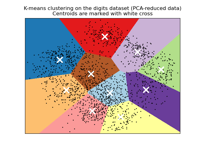
• Inertia is not a normalized metric: we just know that lower values are better and zero is optimal. But in very high-dimensional spaces, Euclidean distances tend to become inflated (this is an instance of the so-called “curse of dimensionality”). Running a dimensionality reduction algorithm such as Principal component analysis (PCA) prior to k-means clustering can alleviate this problem and speed up the computations.

========== picture

K-means is often referred to as Lloyd’s algorithm. In basic terms, the algorithm has three steps. The first step chooses the initial centroids, with the most basic method being to choose k samples from the dataset X. After initialization, K-means consists of looping between the two other steps. The first step assigns each sample to its nearest centroid. The second step creates new centroids by taking the mean value of all of the samples assigned to each previous centroid. The difference between the old and the new centroids are computed and the algorithm repeats these last two steps until this value is less than a threshold. In other words, it repeats until the centroids do not move significantly.

K-means is equivalent to the expectation-maximization algorithm with a small, all-equal, diagonal covariance matrix.

The algorithm can also be understood through the concept of Voronoi diagrams. First the Voronoi diagram of the points is calculated using the current centroids. Each segment in the Voronoi diagram becomes a separate cluster. Secondly, the centroids are updated to the mean of each segment. The algorithm then repeats this until a stopping criterion is fulfilled. Usually, the algorithm stops when the relative decrease in the objective function between iterations is less than the given tolerance value. This is not the case in this implementation: iteration stops when centroids move less than the tolerance.

Given enough time, K-means will always converge, however this may be to a local minimum. This is highly dependent on the initialization of the centroids. As a result, the computation is often done several times, with different initializations of the centroids. One method to help address this issue is the k-means++ initialization scheme, which has been implemented in scikit-learn (use the init='k-means++' parameter). This initializes the centroids to be (generally) distant from each other, leading to probably better results than random initialization, as shown in the reference.

K-means++ can also be called independently to select seeds for other clustering algorithms, see sklearn.cluster.kmeans_plusplus for details and example usage.

The algorithm supports sample weights, which can be given by a parameter sample_weight. This allows to assign more weight to some samples when computing cluster centers and values of inertia. For example, assigning a weight of 2 to a sample is equivalent to adding a duplicate of that sample to the dataset X.

K-means can be used for vector quantization. This is achieved using the transform method of a trained model of KMeans.

Low-level parallelism

KMeans benefits from OpenMP based parallelism through Cython. Small chunks of data (256 samples) are processed in parallel, which in addition yields a low memory footprint. For more details on how to control the number of threads, please refer to our Parallelism notes.

Examples:

• Demonstration of k-means assumptions: Demonstrating when k-means performs intuitively and when it does not
• A demo of K-Means clustering on the handwritten digits data: Clustering handwritten digits

References:

• “k-means++: The advantages of careful seeding” Arthur, David, and Sergei Vassilvitskii, Proceedings of the eighteenth annual ACM-SIAM symposium on Discrete algorithms, Society for Industrial and Applied Mathematics (2007)

Mini Batch K-means

The MiniBatchKMeans is a variant of the KMeans algorithm which uses mini-batches to reduce the computation time, while still attempting to optimise the same objective function. Mini-batches are subsets of the input data, randomly sampled in each training iteration. These mini-batches drastically reduce the amount of computation required to converge to a local solution. In contrast to other algorithms that reduce the convergence time of k-means, mini-batch k-means produces results that are generally only slightly worse than the standard algorithm.

The algorithm iterates between two major steps, similar to vanilla k-means. In the first step, b samples are drawn randomly from the dataset, to form a mini-batch. These are then assigned to the nearest centroid. In the second step, the centroids are updated. In contrast to k-means, this is done on a per-sample basis. For each sample in the mini-batch, the assigned centroid is updated by taking the streaming average of the sample and all previous samples assigned to that centroid. This has the effect of decreasing the rate of change for a centroid over time. These steps are performed until convergence or a predetermined number of iterations is reached.

MiniBatchKMeans converges faster than KMeans, but the quality of the results is reduced. In practice this difference in quality can be quite small, as shown in the example and cited reference.

========= picture

Examples:

• Comparison of the K-Means and MiniBatchKMeans clustering algorithms:
  Comparison of KMeans and MiniBatchKMeans
• Clustering text documents using k-means:
  Document clustering using sparse MiniBatchKMeans
• Online learning of a dictionary of parts of faces

References:

• “Web Scale K-Means clustering”
  D. Sculley, Proceedings of the 19th international conference on
  World wide web (2010)

Affinity Propagation

AffinityPropagation creates clusters by sending messages between pairs of samples until convergence. A dataset is then described using a small number of exemplars, which are identified as those most representative of other samples. The messages sent between pairs represent the suitability for one sample to be the exemplar of the other, which is updated in response to the values from other pairs. This updating happens iteratively until convergence, at which point the final exemplars are chosen, and hence the final clustering is given.

===== picture