aTransformers 1. Introduction 2. Encoder 2.1. Input Embedding 2.2. Positional Encoding 2.3. Encoder Layer 2.4. Multi-Headed Attention 2.5. Residual Connection 2.6. Layer Normalization & Point-wise Feed Forward 3. Decoder 3.1. Output Embedding and Positional Encoding 3.2. First Multi-Headed Attention 3.2.1. Masking 3.3. Second Multi-headed Attention Layer 3.4. Linear Classifier Source 1. Introduction• Transformers are used in many applications like Neural Machine Translation (NMT), conversational chat bots, and search engines.• Why Transformers out-performed models like RNN, GRU, or LSTM?• Some famous examples of Transformer-based models are:– BERT → Bidirectional Encoder Representation from Transformers– GPT → Generative Pre-Training• • Here, we focus on the original architecture of Transformers proposed by the "Attention is All You Need" paper.• • To understand Transformers, we must first understand the Attention Mechanism.• To get an intuitive understanding of the attention mechanism, let's start with a text generation model that's capable of writing its own sci-fi novel.• We need to prompt the model with an arbitrary input and the model will generate the rest.

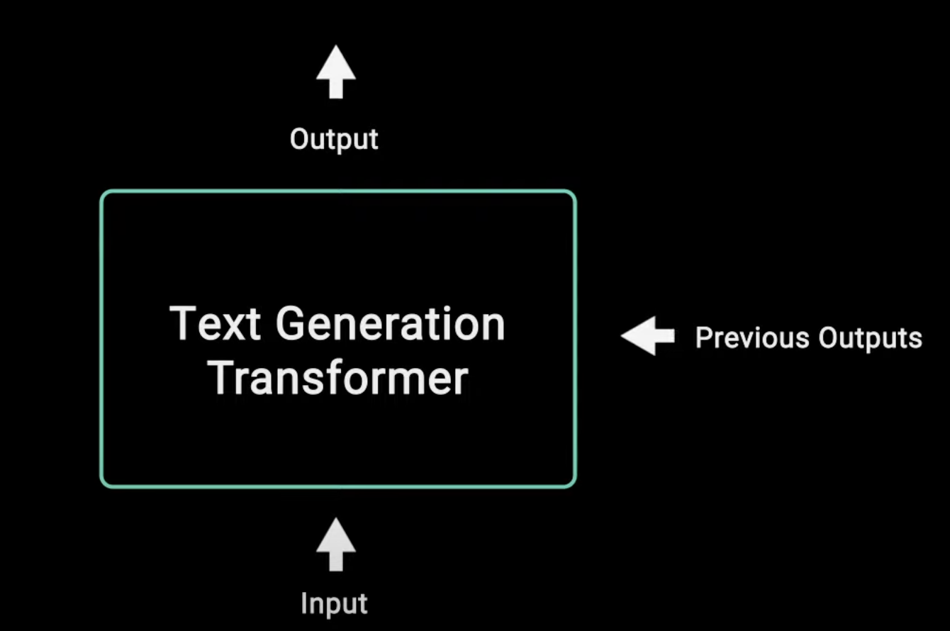
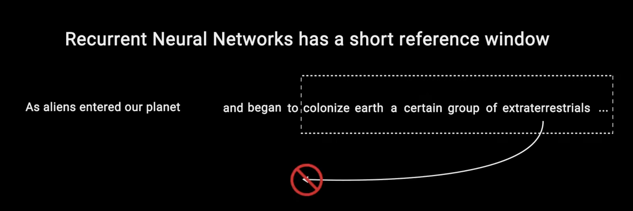
• So how it works?– As the model generate text word by word, it has the ability to reference or tend to words that's relevant to the generated word. – How the model knows where to attend to is all learned while training via backpropagation. – • RNNs are also capable of looking at previous inputs too. But the power of the attention mechanism is that it doesn't suffer from short-term memory.• RNNs have a shorter window to reference from → so, when the story gets longer, RNNs can't access word generated earlier in the sequence.

Figure 1:RNNs have short memory

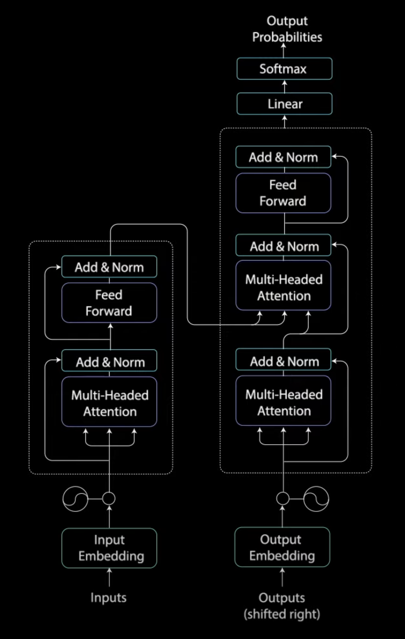
• This is also true for GRU and LSTM → Although they do have a bigger capacity to achieve longer term memory → Therefore, having a longer window to reference from.• • The attention mechanism in theory, and given enough compute resources, have an infinite window to reference from.– Therefore, being capable of using the entire context of the story while generating the text. • This power was demonstrated in the "Attention is All You Need" paper, when the authors introduced a new novel neural network called the Transformers, which is an attention-based encoder decoder type architecture.

Figure 2:Transformer

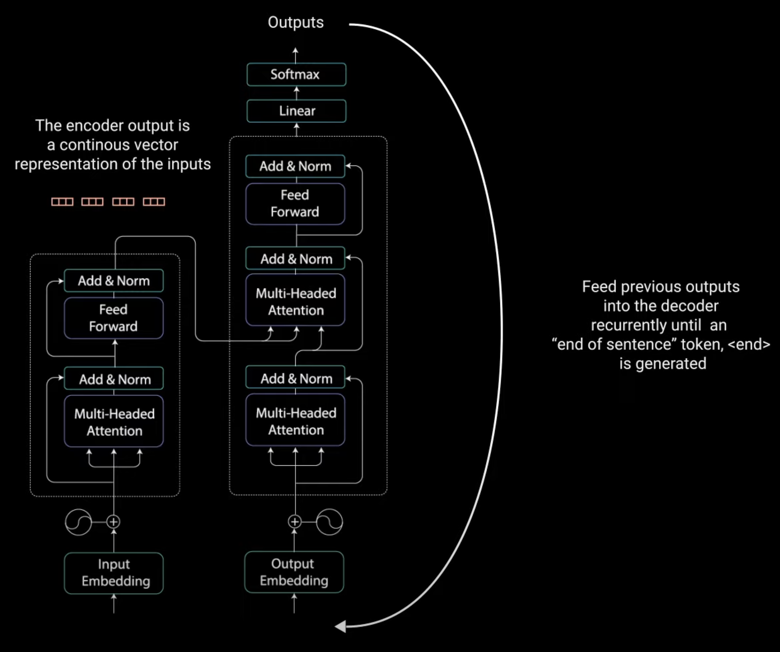
• On a high level, the encoder maps an input sequence into an abstract continuous representation that holds all the learned information of that input.• The decoder, then takes that continuous representation and step by step generates a single output while also being fed to previous output.

Figure 3:Transformer Architecture

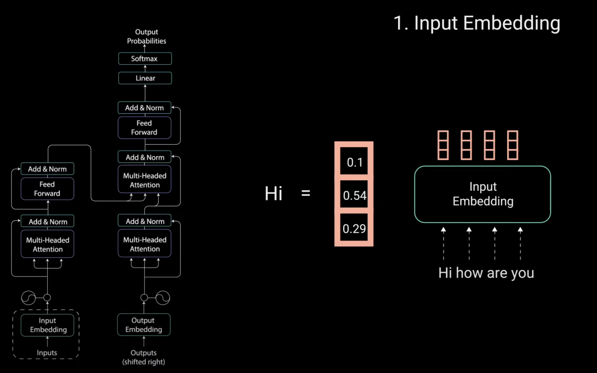
• The paper applied the Transform model on a NMT. Our demonstration of the Transformer model would be a conversational chat bot. It takes an input text, and generate a response. 2. Encoder2.1. Input Embedding• The first step is feeding our input into a word Embedding Layer. • A word embedding layer can be thought of as a lookup table to grab a learned representation of each word.• Neural networks learn through numbers so each word maps to a vector with continuous values to represent that word.

Figure 4:Word Embedding Layer

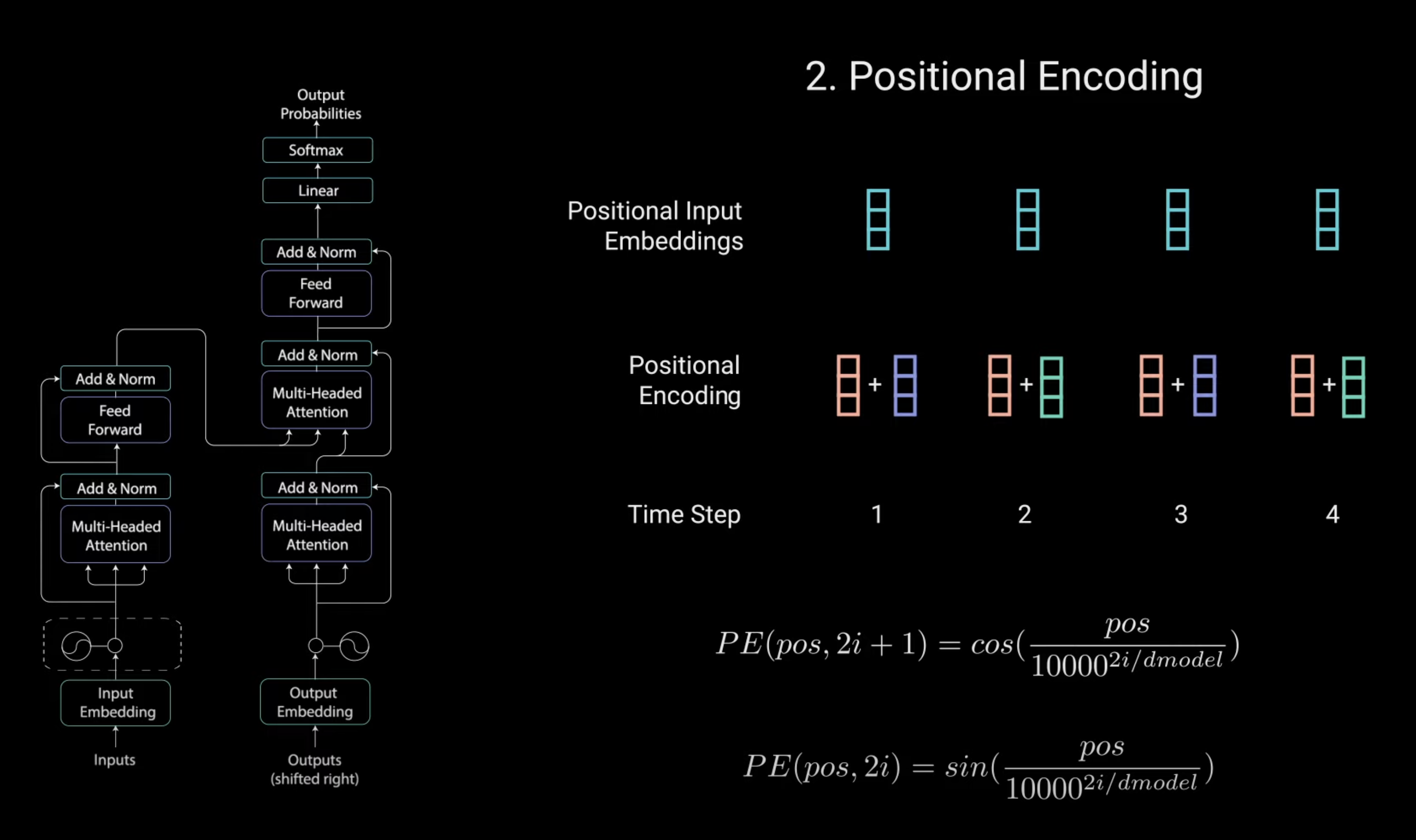
2.2. Positional Encoding• Next step is to to inject positional information into the embeddings.• Because a Transformer encoder has no recurrence (like RNN), we must add information about the positions into the input embeddings.• This is done using positional encoding.• The authors of the original paper came up with a clever trick using sine and cosine functions. To put it simply:– For every odd time step, create a vector using the cosine function.– For every even time step, create a vector using the sine function.– Then, add those vectors to their corresponding embedding vector.• This successfully gives the network information on the positions of each vector.• The sine and cosine functions were chosen in tandem because they have linear properties the model can easily learn to attend to.

Figure 5:Positional encoding

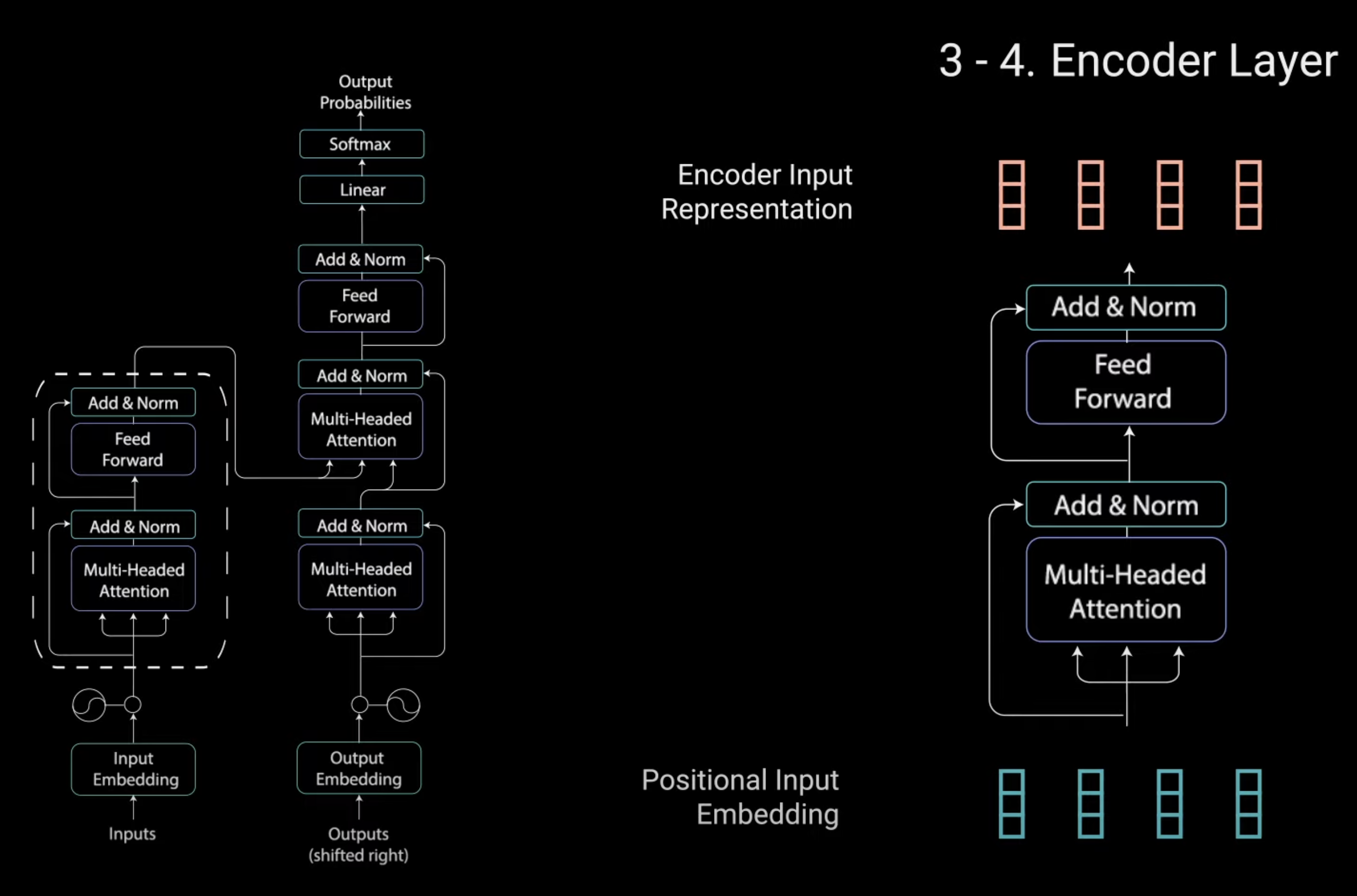
2.3. Encoder Layer• The encoder layer's job is to map all input sequence into an abstract continuous representation that holds the learned information for that entire sequence.• It contains two sub modules.– Multi-headed Attention– Fully-Connected Layer• There are also Residual Connections around each of the two sub modules followed by a Layer Normalization.•

Figure 6:Transformer Encoder

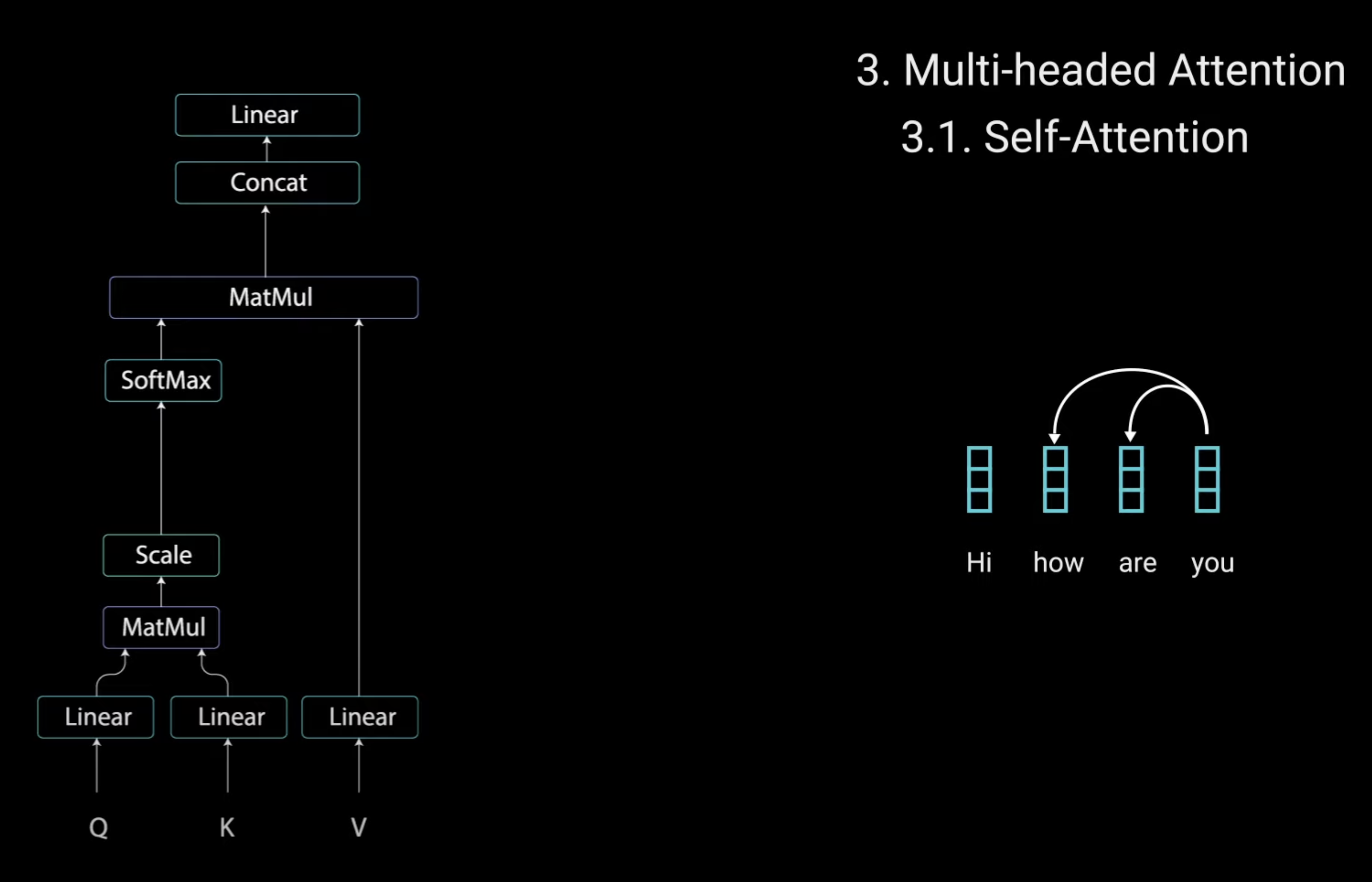
2.4. Multi-Headed Attention• Multi-headed Attention in the encoder applies a specific attention mechanism called Self-Attention.• Self-Attention allows a model to associate each individual word in the input to other words in the input.– In the example → "Hi, how are you?", it's possible that our model can learn to associate the word "you" with "how" and "are". – It's also possible that the model learns that word structured in this pattern are typically a question so respond appropriately.

Figure 7:Self-Attention

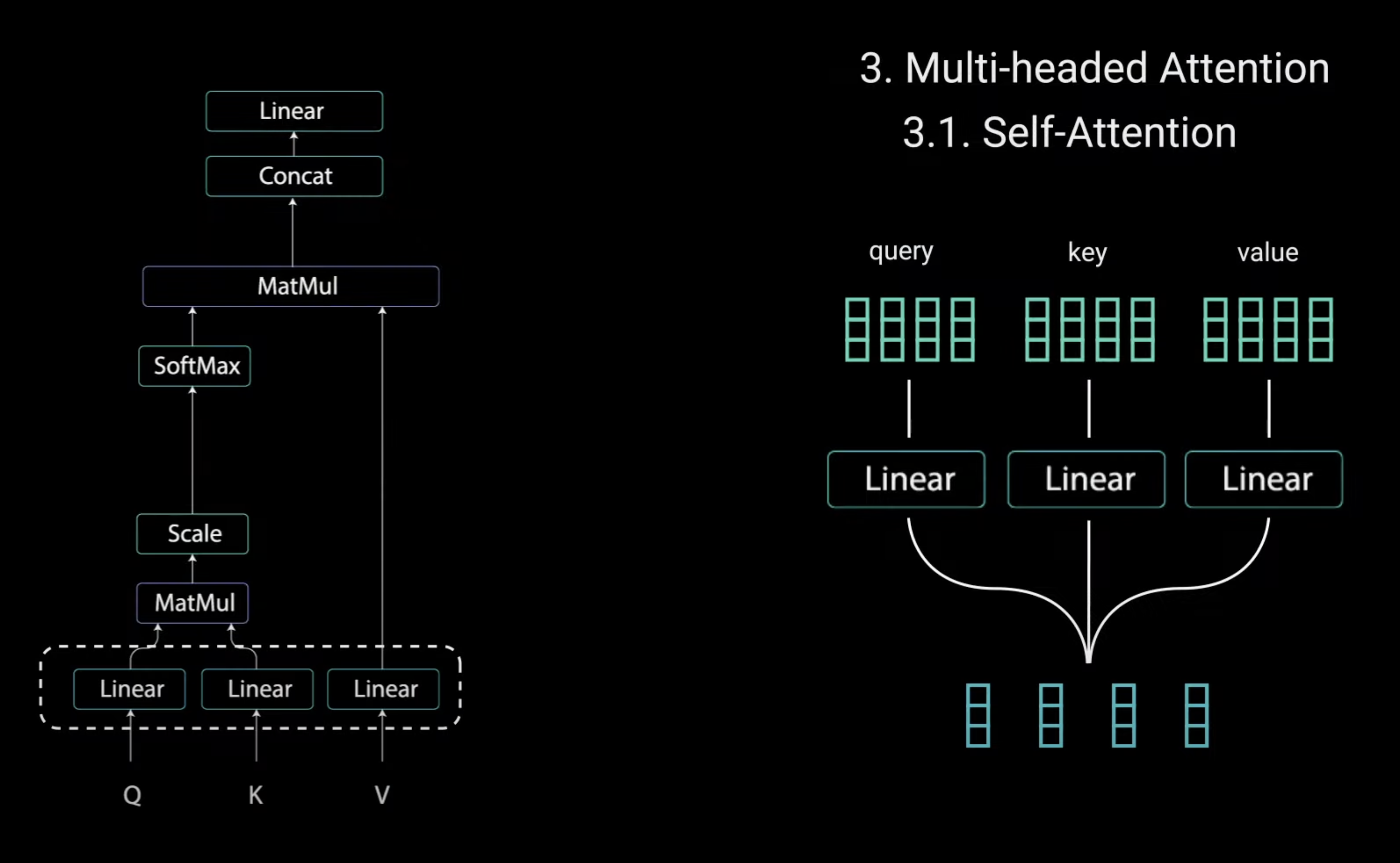
• To achieve Self-Attention, we feed the input into three distinct fully connected layers to create the query, key, and value vectors.

Figure 8:Query, Key, and Value in Self-Attention

• What are these vectors exactly?– The query/key/value concepts come from retrieval systems. – For example, * When you type a query to search for some video on YouTube, the search engine will map your query against a set of keys (video title, description, etc.) associated with candidate videos in the database, then present you the best matched video (value).– The attention operation can be thought of as a retrieval process as well.– As mentioned in the paper you referenced (Neural Machine Translation by Jointly Learning to Align and Translate), attention by definition is just a weighted average of values,c= ∑j𝛼jhj$$c=\sum _j^{}{𝛼}_j{h}_j$$• – where ∑𝛼j=1${\displaystyle \sum {𝛼}_j=1}$.– If we restrict 𝛼${\displaystyle 𝛼}$ to be a one-hot vector, this operation becomes the same as retrieving from a set of elements h${\displaystyle h}$ with index 𝛼${\displaystyle 𝛼}$. – With the restriction removed, the attention operation can be thought of as doing "proportional retrieval" according to the probability vector 𝛼${\displaystyle 𝛼}$.– It should be clear that h${\displaystyle h}$ in this context is the value. – The difference between the two papers lies in how the probability vector 𝛼${\displaystyle 𝛼}$ is calculated. – The first paper (Bahdanau et al. 2015) computes the score through a neural network– eij=a(si,hj) 𝛼i,j=eeij

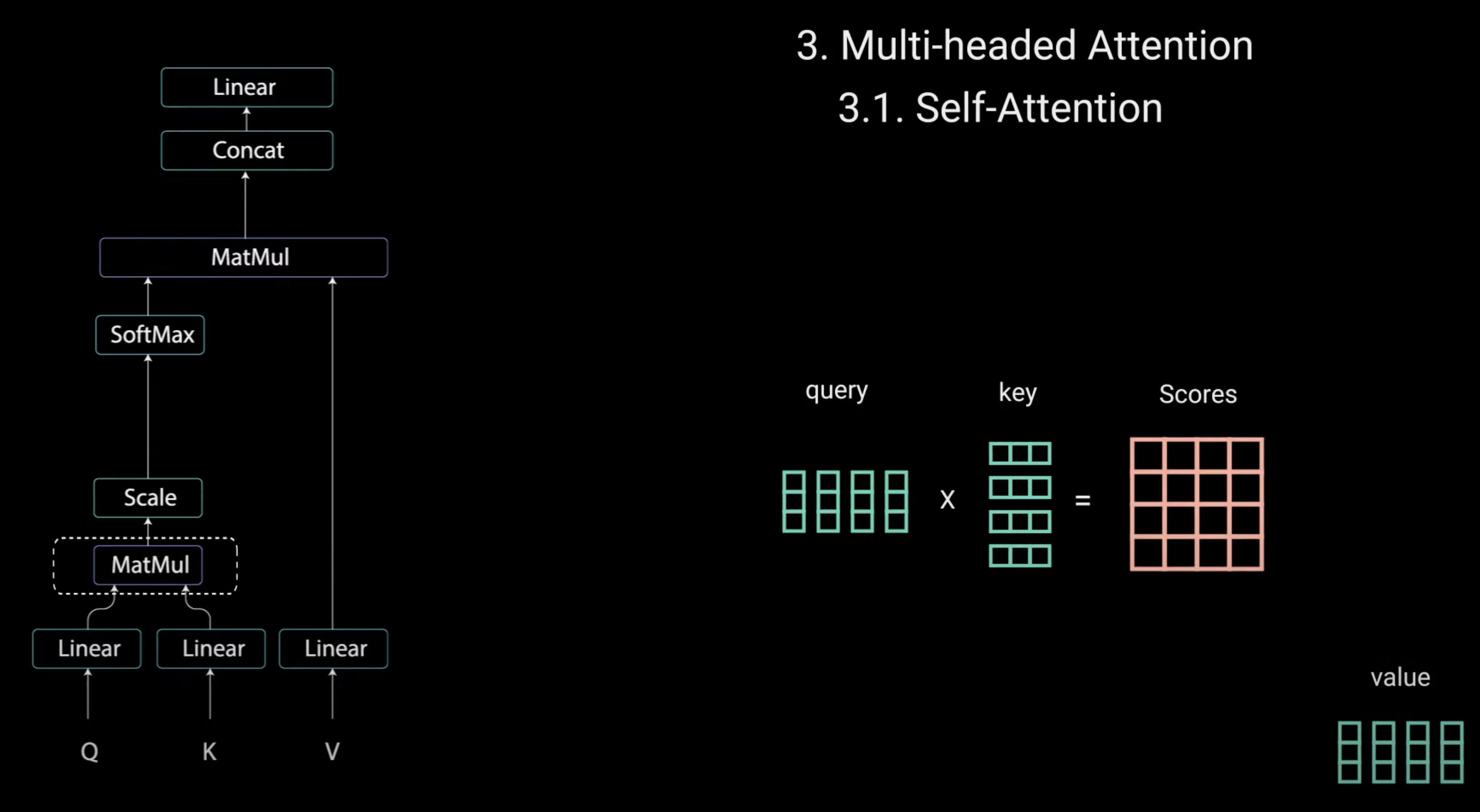
∑keeik$$e_{ij}=a(s_i,h_j){𝛼}_{i,j}=\frac{e^{e_{ij}}}{\sum _k^{}{e}_{}^{e_{ik}}}$$• – where hj${\displaystyle h_j}$ is from the encoder sequence, and si${\displaystyle s_i}$ is from the decoder sequence. – One problem of this approach is, say the encoder sequence is of length m${\displaystyle m}$ and the decoding sequence is of length n${\displaystyle n}$, we have to go through the network m×n${\displaystyle m\times n}$ times to acquire all the attention scores eij${\displaystyle e_{ij}}$.– A more efficient model would be to first project s${\displaystyle s}$ and h${\displaystyle h}$ onto a common space, then choose a similarity measure (e.g. dot product) as the attention score, like– eij=f(si)g(hj)T$$e_{ij}=f(s_i)g(h_j{)}^T$$• – So, we only have to compute g(hj)${\displaystyle g(h_j)}$ m${\displaystyle m}$ times and f(si)${\displaystyle f(s_i)}$ n${\displaystyle n}$ times to get the projection vectors and eij${\displaystyle e_{ij}}$ can be computed efficiently by matrix multiplication.– This is essentially the approach proposed by the second paper (Vaswani et al. 2017), where the two projection vectors are called query (for decoder) and key (for encoder), which is well aligned with the concepts in retrieval systems. (There are later techniques to further reduce the computational complexity, for example Reformer, Linformer.) • How are the queries, keys, and values obtained?– The proposed Multi-Head Attention alone doesn't say much about how the queries, keys, and values are obtained, they can come from different sources depending on the application scenario.– MultiHead(Q,K,V)=Concat(head1,…,headn)Wo where headi=Attention(QWQi,KWKi,VWVi) WQi∈Rdmodel×dkWKi∈Rdmodel×dkWVi∈Rdmodel×dvWOi∈Rhdv×dmodel$$\begin{array}{c}\text{MultiHead}(Q,K,V)=\text{Concat}({\text{head}}_1,\dots ,{\text{head}}_n)W^o\\ \\ \text{where}{\text{head}}_i=\text{Attention}(Q{W}_i^Q,K{W}_i^K,V{W}_i^V)\\ \\ W_i^Q\in {\mathbb{R}}^{d_{model}\times d_k}\\ W_i^K\in {\mathbb{R}}^{d_{model}\times d_k}\\ W_i^V\in {\mathbb{R}}^{d_{model}\times d_v}\\ W_i^O\in {\mathbb{R}}^{h{d}_v\times d_{model}}\end{array}$$• – For unsupervised language model training like GPT, Q,V,K${\displaystyle Q,V,K}$ are usually from the same source, so such operation is also called self-attention.– For the machine translation task in the second paper, it first applies self-attention separately to source and target sequences, then on top of that it applies another attention where Q${\displaystyle Q}$ is from the target sequence and K,V${\displaystyle K,V}$ are from the source sequence.– For recommendation systems, Q${\displaystyle Q}$ can be from the target items, K,V${\displaystyle K,V}$ can be from the user profile and history.• • The queries and keys undergo a dot product matrix multiplication to produce a score matrix.

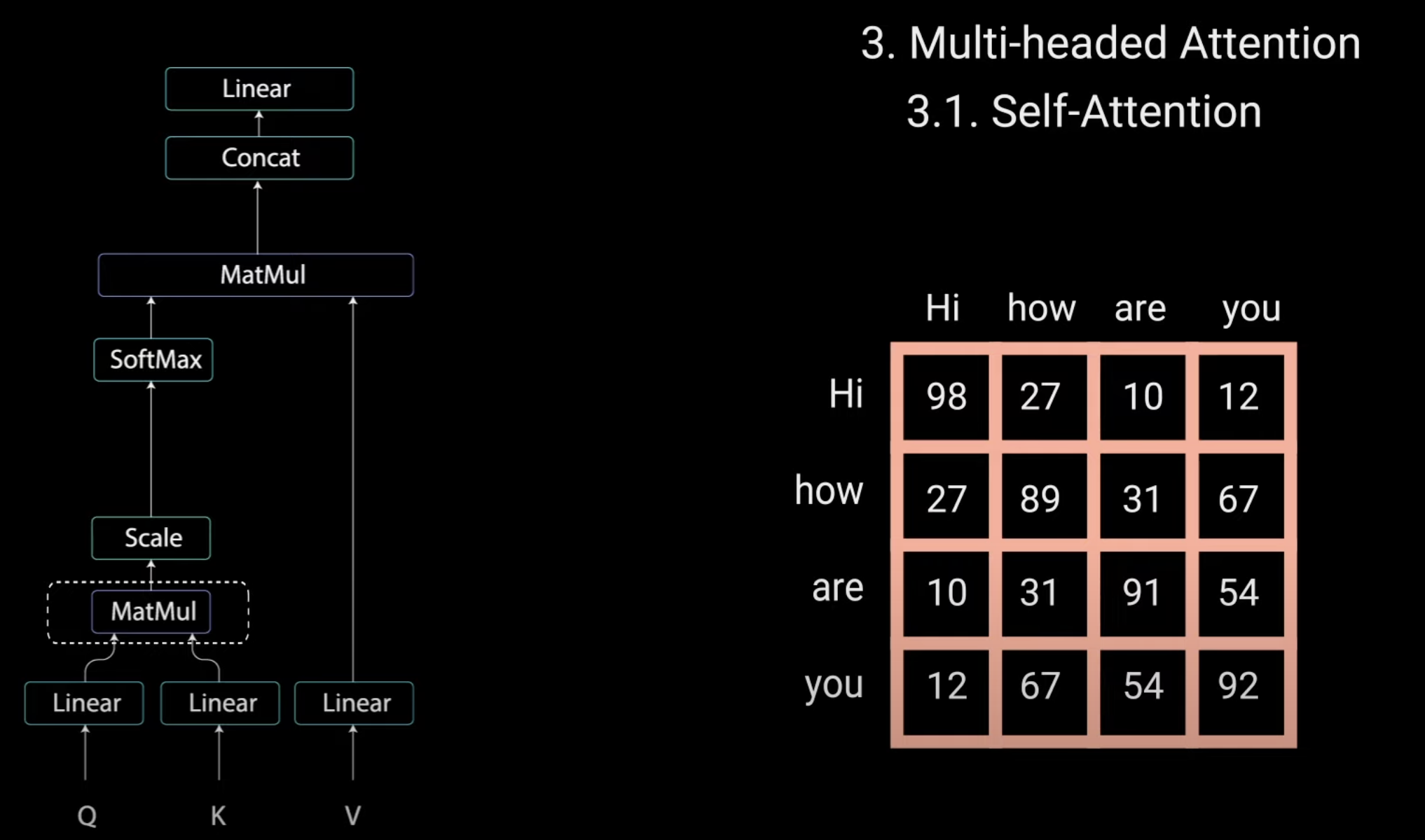
Figure 9:Word association score matrix

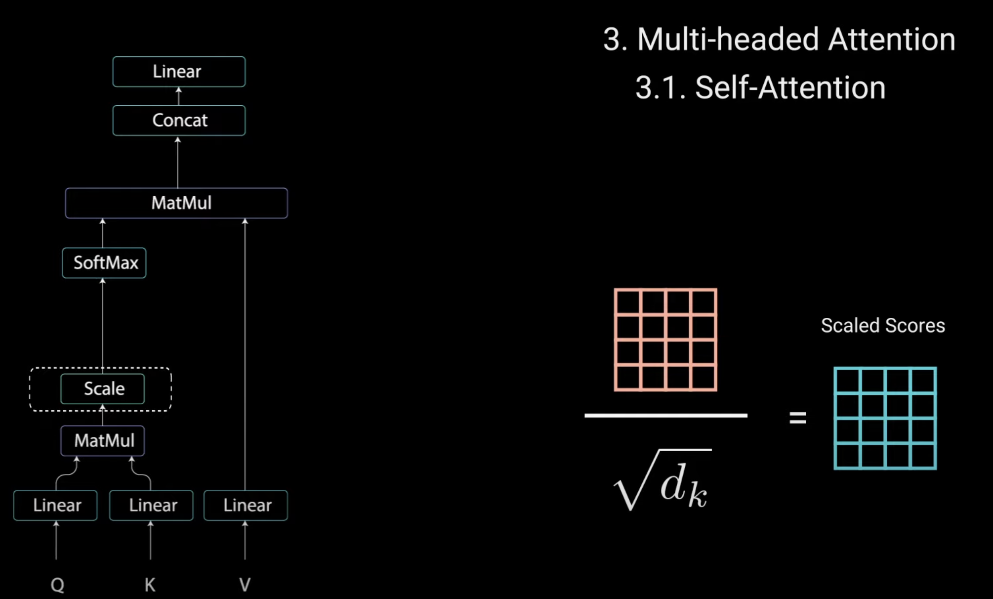
• The score matrix determines how much focus should a word be put on other words. – So, each word will have score that correspond to other words in the time step.– The higher the score, the more the focus. This is how queries are mapped to keys. • • Then the scores get scaled down by getting divided by the square root of the dimension of the queries and the keys.– This is to allow for more stable gradients as multiplying values can have exploding effects.

Figure 10:Scaling association scores

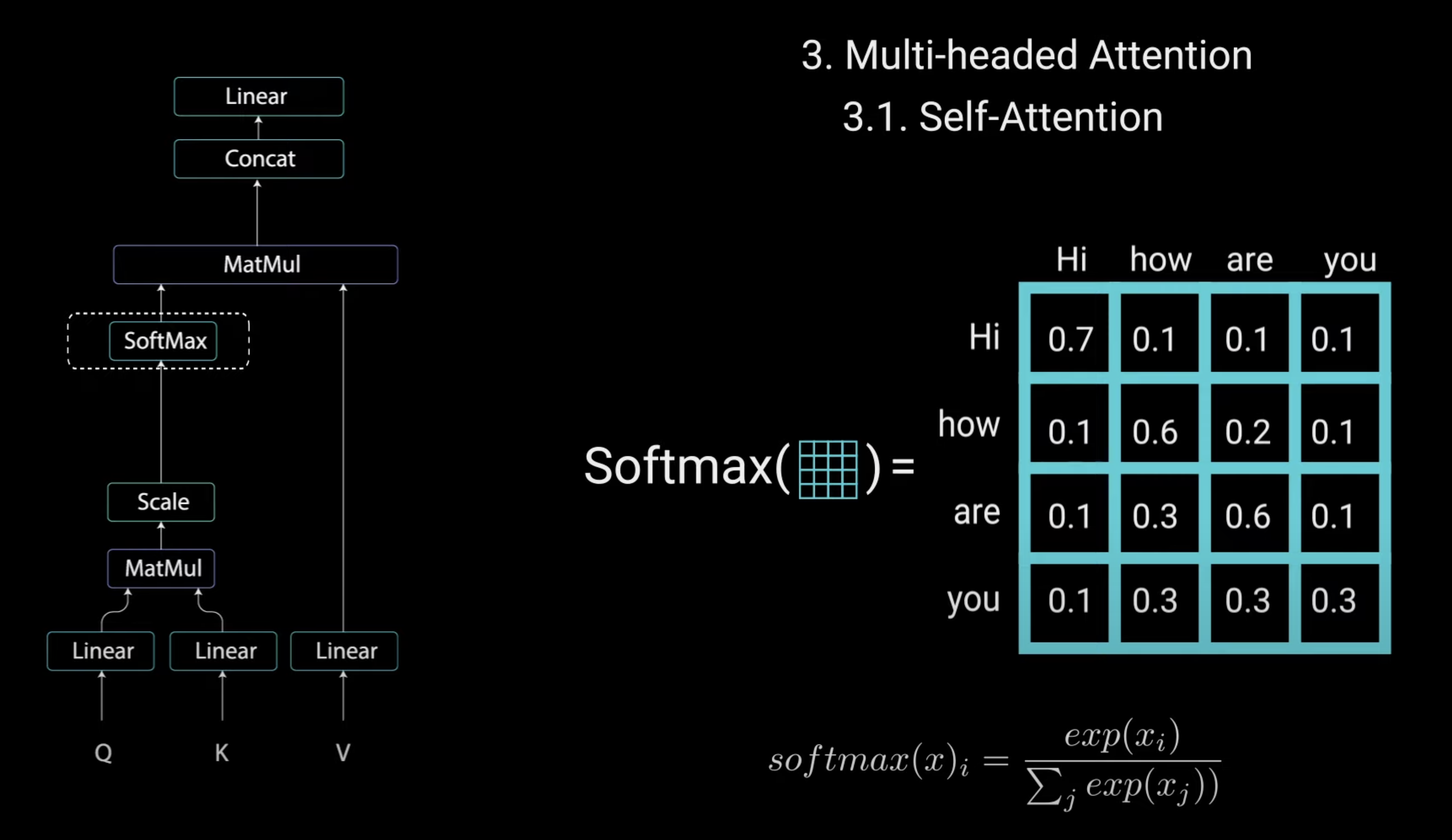
• Next, you take the softmax of the scaled scores to get the attention weights which gives probability values between 0 and 1.• By doing a softmax, the higher scores get heightened and the lower scores are depressed.– This allows the model to be more confident on which words to attend to.

Figure 11:Applying softmax to association scores

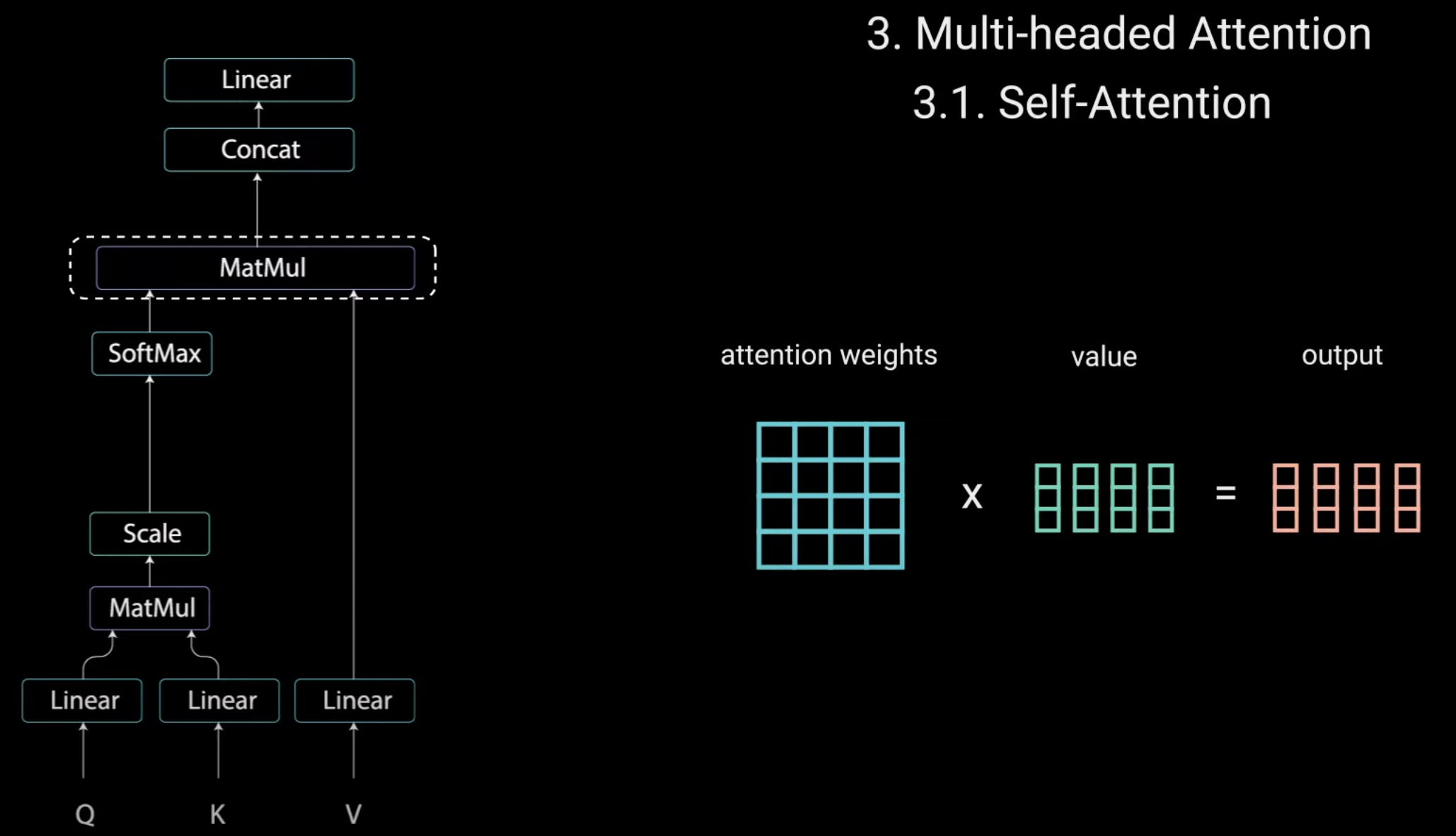
• Then, you take the attention weights and multiply it by your value vector to get an output vector. – The higher softmax scores will keep the value of the words that the model learn as more important. The lower scores will drown out the irrelevant words.• You feed the output vector into a Linear Layer to process.

Figure 12:Getting the output (value) vector

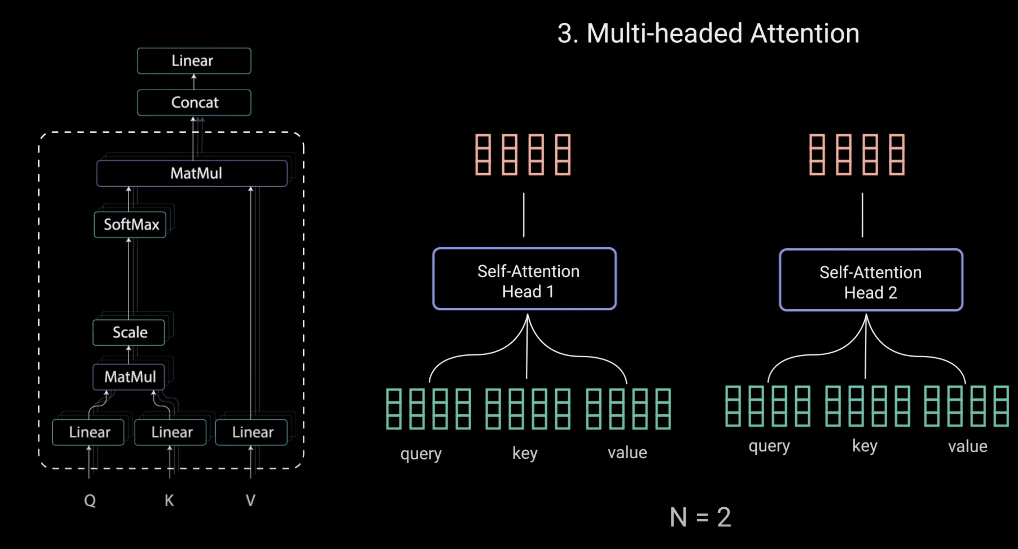
• To make this a Multi-headed Attention computation, you need to split the query, key, and value into n${\displaystyle n}$ vectors before applying Self-Attention.• The split vectors then go through the same Self-Attention process individually.

Figure 13:Heads of Multi-headed Attention

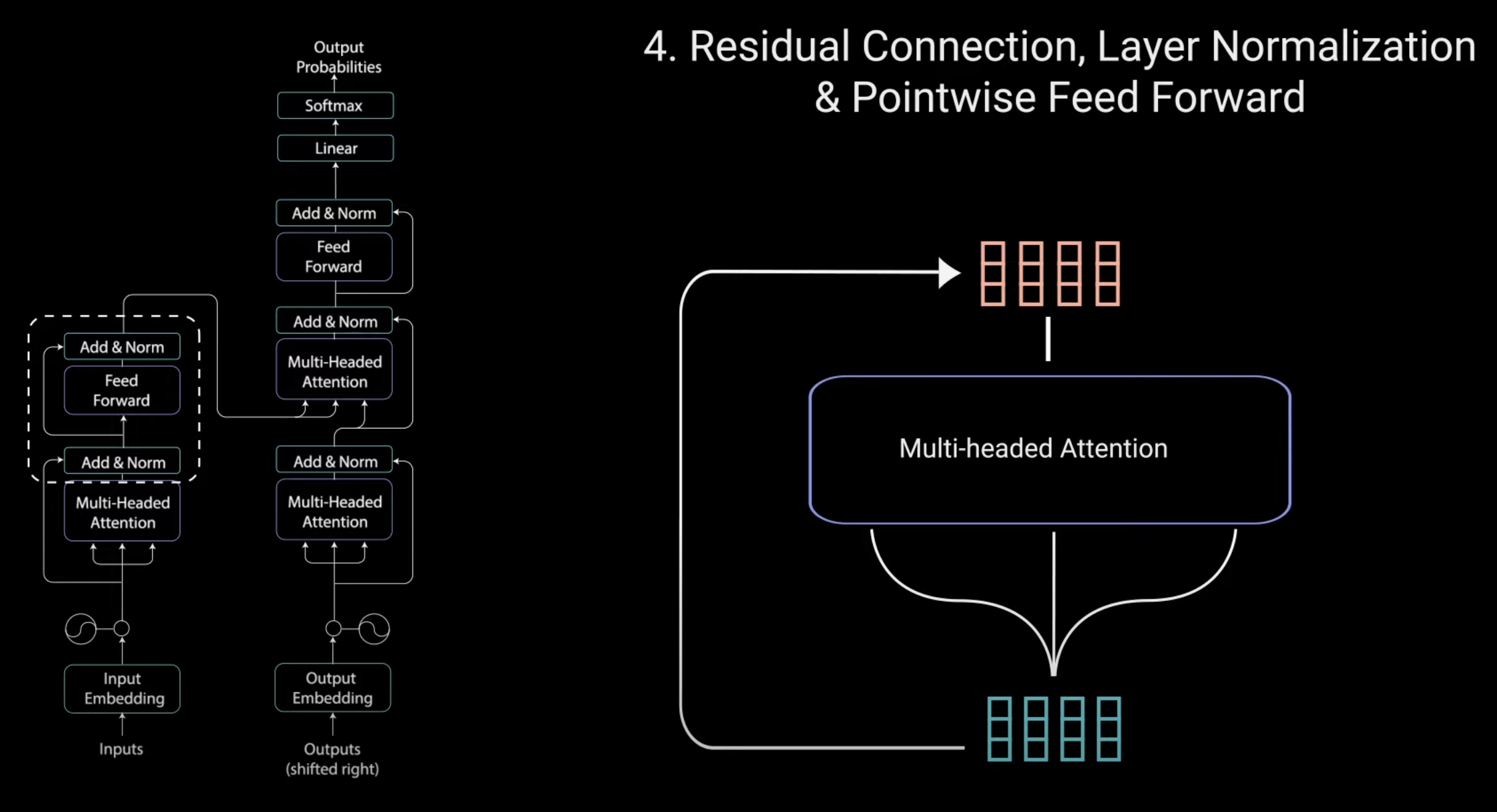
• Each Self-Attention process is called a head.– Each head produces an output vector that gets concatenated into a single vector before go through the final linear layer.– In theory, each head would learn something different, therefore, giving the encoder model more representation power.• • To sum it up, Multi-headed Attention is a module in a Transformer network that computes the attention weights for the input and produces an output vector with encoded information on how each word should attend to all other words in a sequence.• 2.5. Residual Connection• Next step, the Multi-headed Attention output vector is added to the original input.• This is called a Residual Connection.

Figure 14:Residual Connections in the Encoder

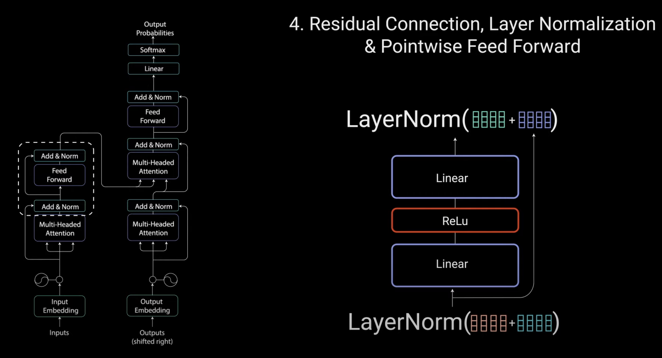
2.6. Layer Normalization & Point-wise Feed Forward• The output of the Residual Connection goes through a Layer Normalization.• The normalized residual output gets fed into a Point-wise Feed-Forward network for further processing.• The Point-wise Feed-Forward network are a couple of Linear Layers with ReLU activation in between.• The output of that is again added to the input of the Point-wise Feed-Forward network and further normalized.• The Residual Connections helps the network train by allowing gradients to flow through the networks directly.• The Layer Normalization are used to stabilize the network which results in substantially reducing the training time necessary.• A Point-wise Feed-Forward layer are used to further process the attention output potentially giving it a richer representation.

Figure 15:Layer Normalization

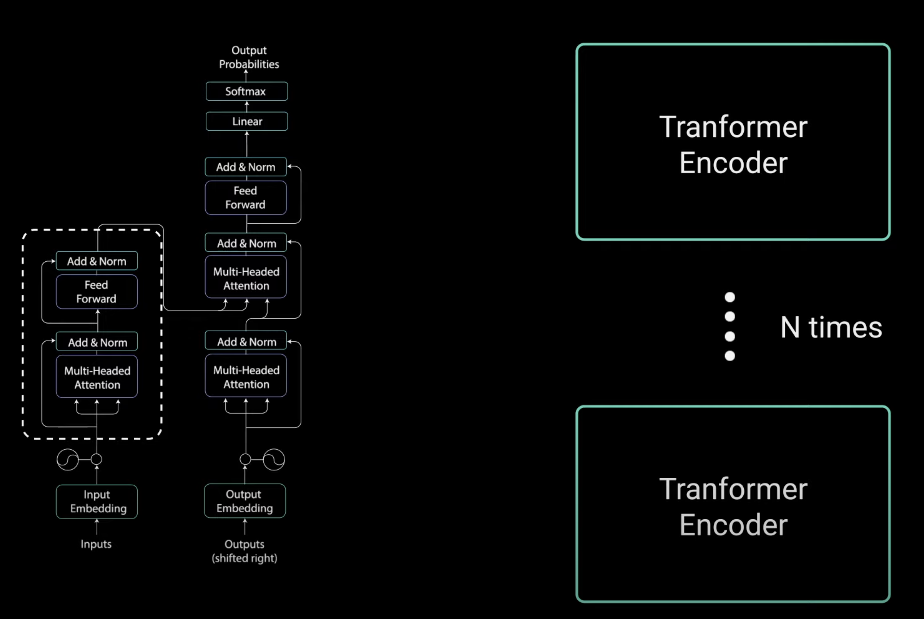
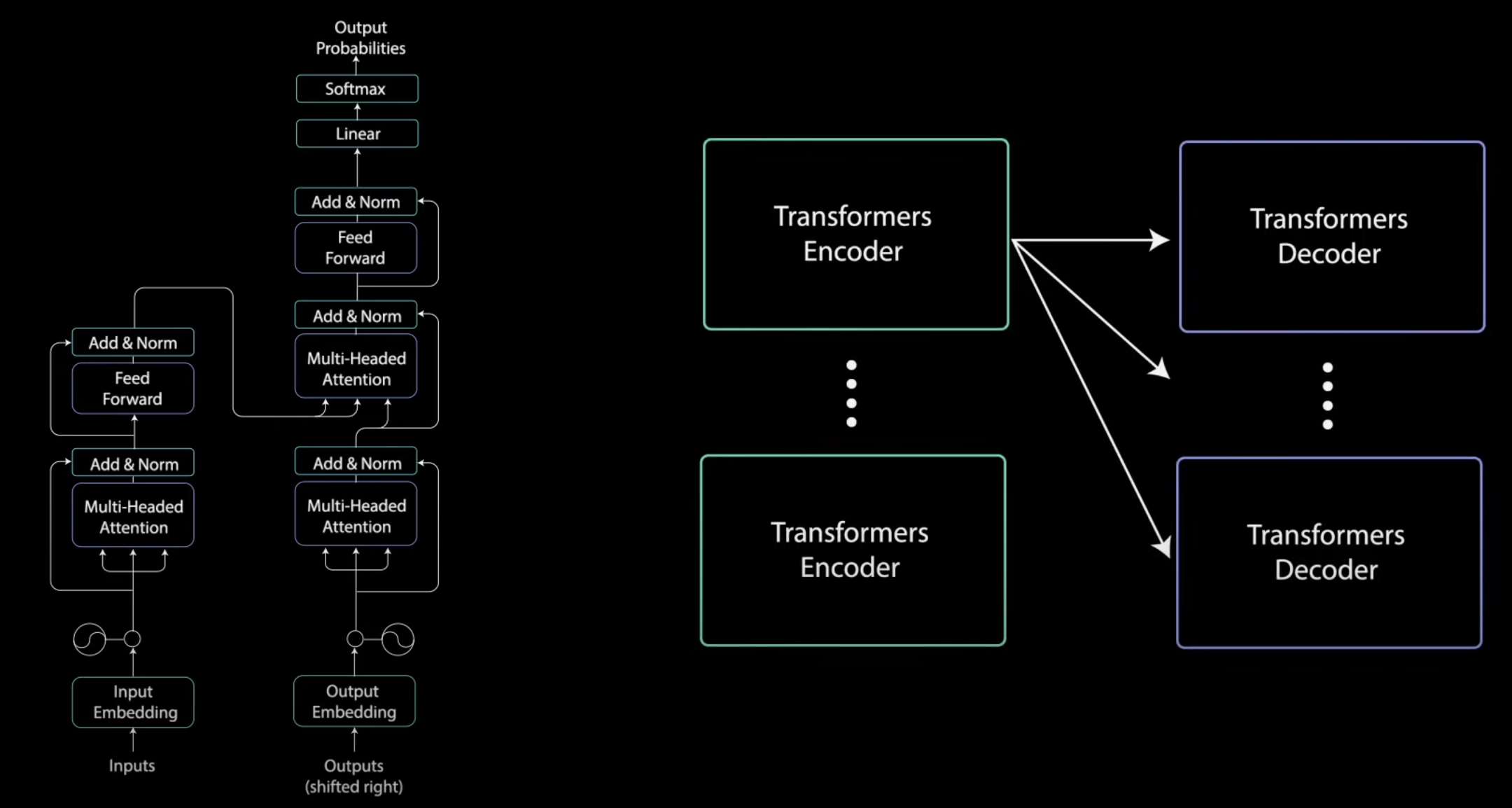
• This wraps up the Encoder Layer → These operations is for the purpose encoding the input to a continuous representation with attention information → This will help the Decoder focus on the appropriate words in the input during the decoding process.• You can stack the Encoder N${\displaystyle N}$ times to further encode the information where each layer has the opportunity to learn different attention representations → Therefore, potentially, boosting the predictive power of the transformer network.

Figure 16:Stacking N${\displaystyle N}$ Transformer Encoders

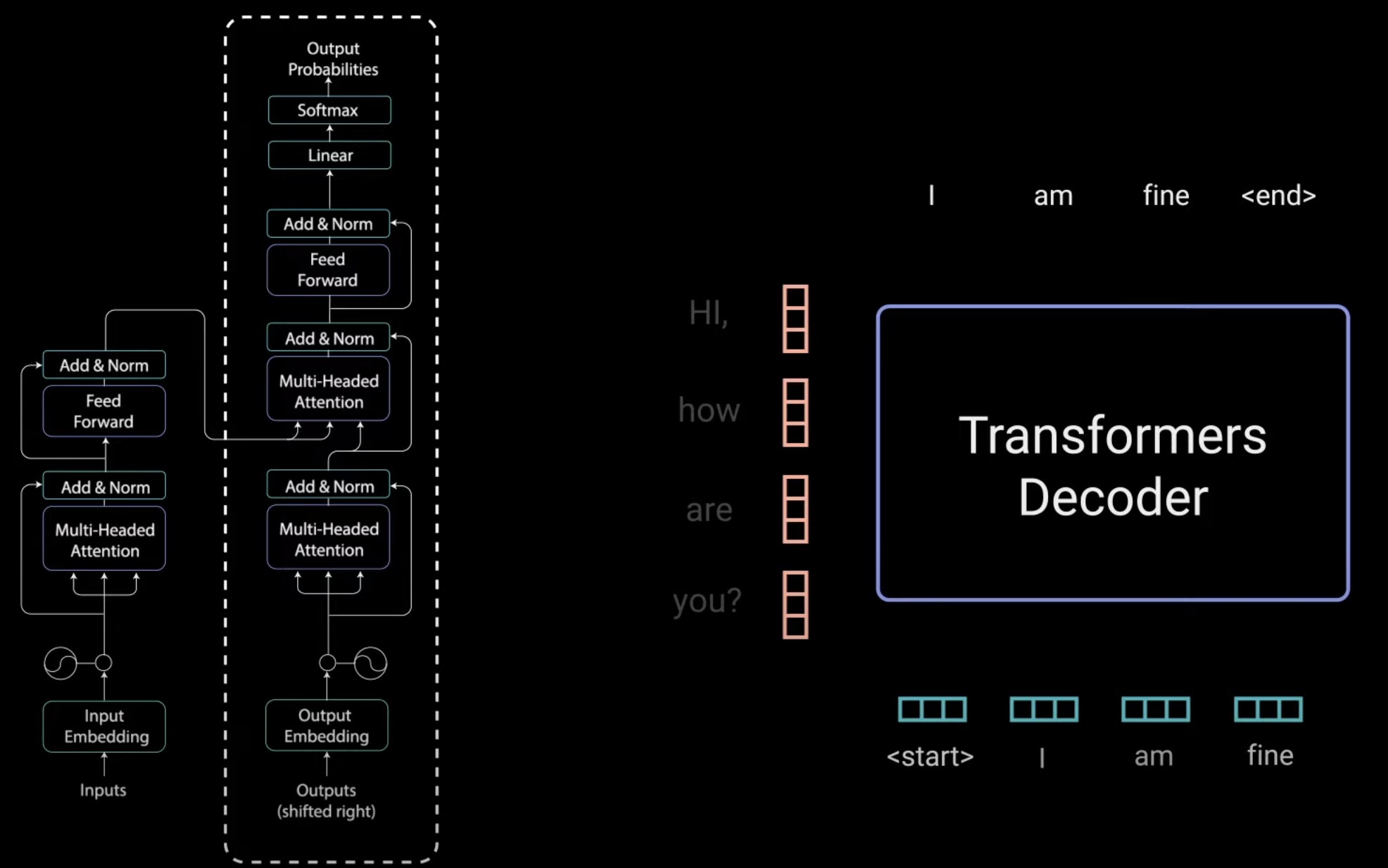
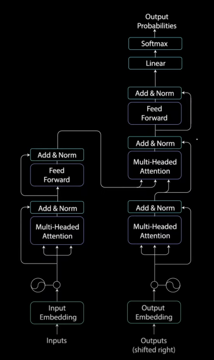
3. Decoder• The Decoder's job is to generate text sequences.• The decoder has similar sub layers as the Encoder.• It has two Multi-headed Attention layers, a Point-wise Feed-Forward layer with Residual Connections and Layer Normalization after each sub layer.• These sub layers behave similarly to layers in the Encoder but each Multi-headed Attention layer has different job.• Decoder is capped off with a Linear Layer that acts like a classifier and a softmax to get the word probabilities.

Figure 17:Transformer Decoder

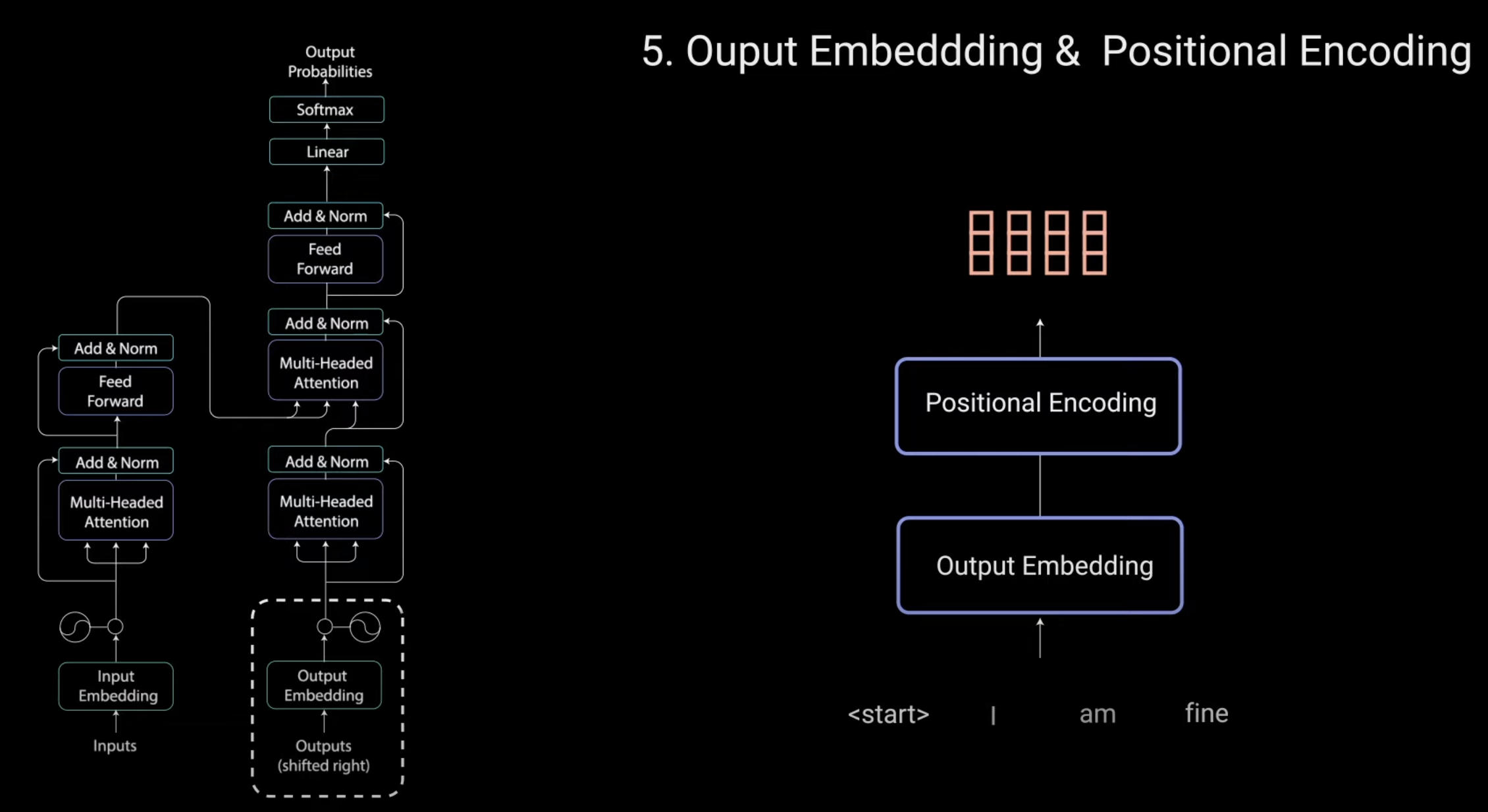
• The Decoder is auto-regressive.– It takes in the list of previous outputs as inputs as well as the Encoder's outputs that contains the attention information from the input.• The Decoder stops decoding when it generates and <end> token as an output. 3.1. Output Embedding and Positional Encoding• The input goes through an Embedding Layer in a Positional Encoding Layer to get positional embeddings.

Figure 18:Positional Encoding

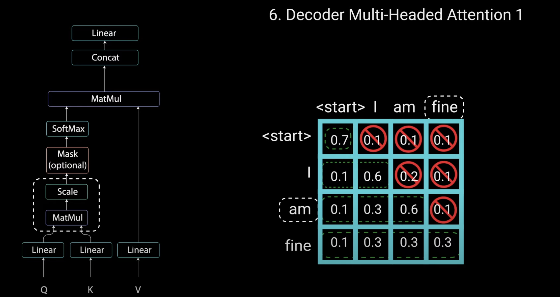
3.2. First Multi-Headed Attention• The positional embeddings get fed into the first Multi-headed Attention Layer which computes the attention score for the Decoder's input.• This Multi-headed Attention operates slightly different → Since the Decoder is auto-regressive and generates the sequence word-by-word, you need to prevent it from condition into future tokens.– For example, when computing attention scores on the word "am", you should not have access to the word "fine", because that word is a future word that was generated after.– The word "am" should only have access to itself and the words before.– This is true for all other words where they can only attend to to previous words.

Figure 19:Masking

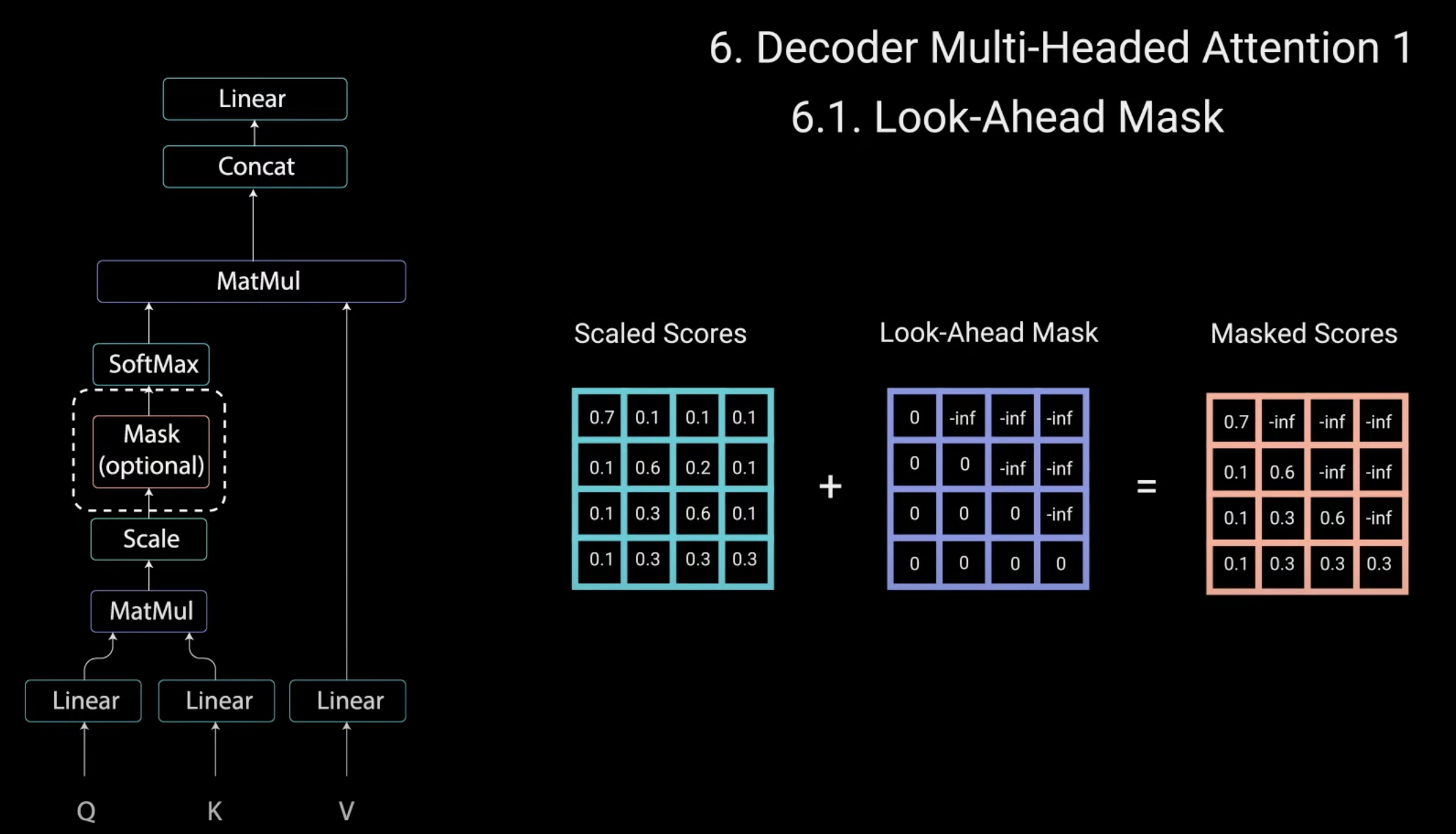
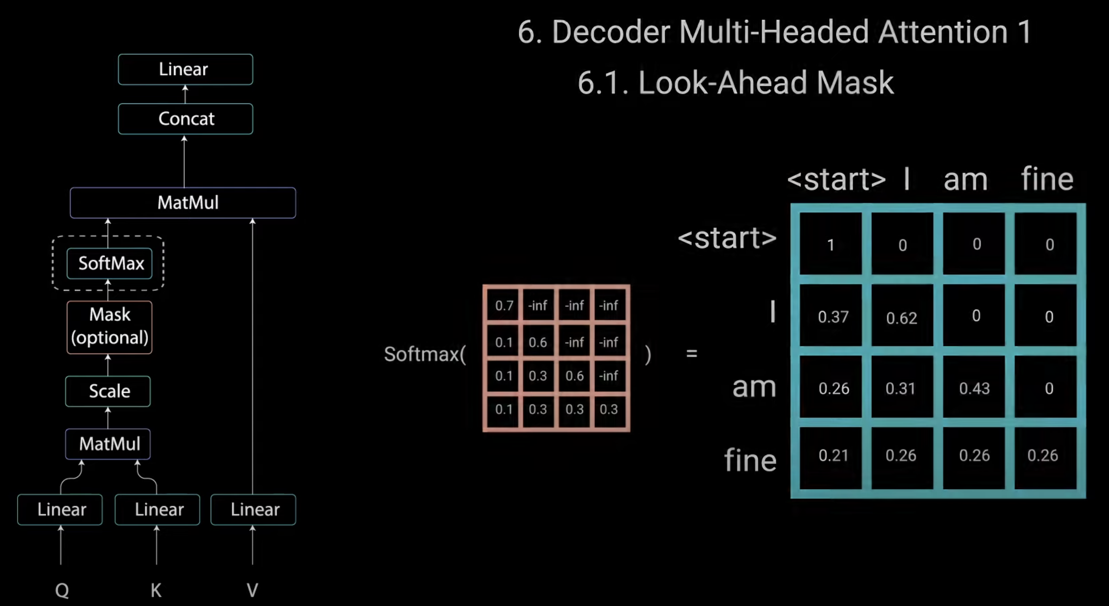
3.2.1. Masking• We need a method to prevent computing attention scores for future words. • This method is called masking.• To prevent the Decoder from looking at future tokens you apply a look-ahead mask.• The mask is added before calculating the softmax and after scaling the scores.• Let's see how this works.– The mask is a matrix that's the same size as the attention scores, filled with values of 0${\displaystyle 0}$s and -inf. – When you add the mask to the scaled attention scores, you get a matrix of scores the top right triangle filled with -inf.– The reason for this is once you take the softmax the masked scores, the -inf get zeroed out, leaving a zero attention score for future tokens.– This tells the model to put no focus on the future tokens.

Figure 20:Look-ahead Masks

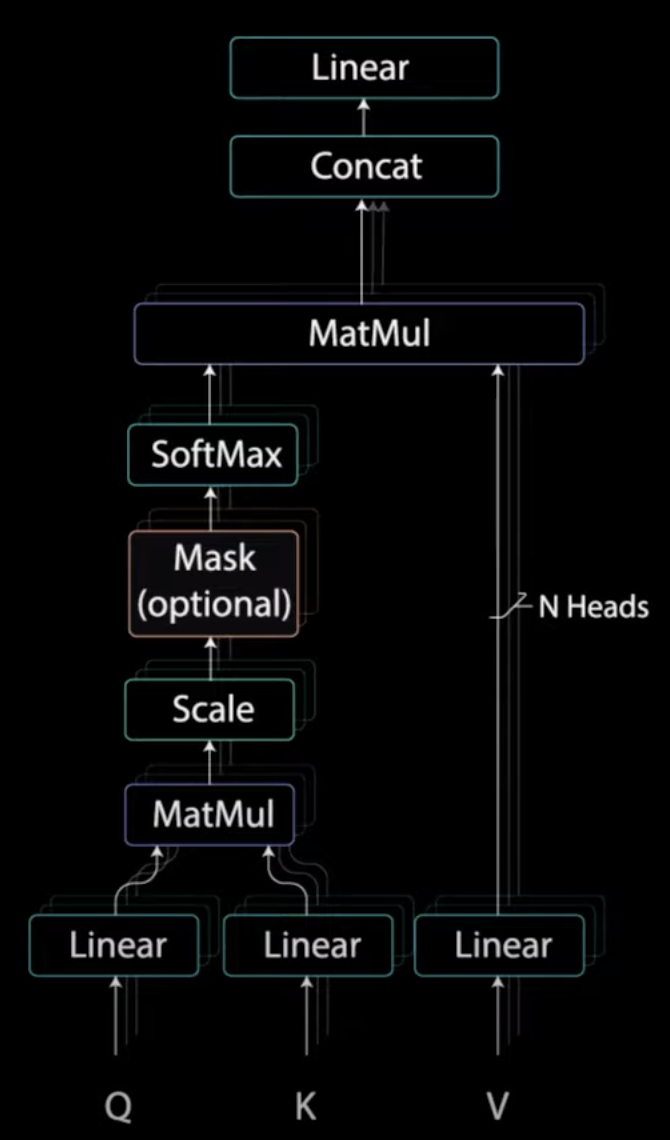
• Masking is the only difference on how the attention scores are calculated in the first Multi-headed Attention Layer.• This layer still have multiple heads that the mask are being applied to before getting concatenated and fed through Linear Layer for further processing.•

Figure 21:The First Multi-headed Attention Layer in Decoder

• The output of the first Multi-headed Attention is a mask output vector with information on how the model should attend on the decoders inputs. 3.3. Second Multi-headed Attention Layer• For this layer the Encoder's output are the queries and the keys, and the first Multi-headed Attention Layer outputs are the values.• This process matches the Encoder's input to the Decoder's input allowing the Decoder to decide which Encoder input is relevant to put focus on.• The output of the second Multi-headed Attention Layer goes through a Point-wise Feed-Forward layer for further processing.

Figure 22:The Second Multi-headed Attention Layer in Decoder

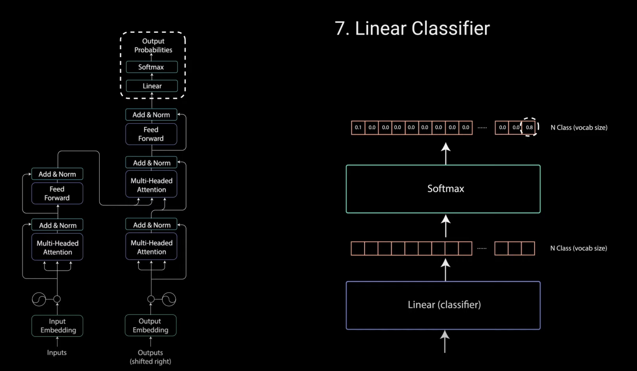
3.4. Linear Classifier• The final Point-wise Feed Forward layer's output goes through a final Linear Layer that access a classifier.• The classifier is as big as the number of classes you have.– For example, if you have 10,000 classes for 10,000 words, the output of that classifier will be of size 10,000.– The output of the classifier again gets fed into a softmax function to produce probability scores for each class. – We take in the index of the highest probability and that equals our predicted word.

Figure 23:Linear Classifier

• The Decoder then takes the output and adds it to the list of Decoder inputs and continue decoding until <end> token is predicted.• The Decoder can also be stacked N${\displaystyle N}$ times with each layer taking in inputs from the Encoder and the layers before it.• By stacking layers the model can learn to extract and focus on different combinations of attention from its attention heads, potentially, boosting its predictive power.

Figure 24:Stacking Decoder N${\displaystyle N}$ times